Introduction
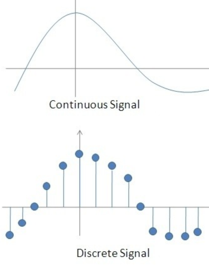
Time series provide the opportunity to forecast future values. Based on previous values, time series can be used to forecast trends in economics, weather, and capacity planning, to name a few. The specific properties of time-series data mean that specialized statistical methods are usually required.
In this tutorial, we will aim to produce reliable forecasts of time series. We will begin by introducing and discussing the concepts of autocorrelation, stationarity, and seasonality, and proceed to apply one of the most commonly used method for time-series forecasting, known as ARIMA.
One of the methods available in Python to model and predict future points of a time series is known as SARIMAX, which stands for Seasonal AutoRegressive Integrated Moving Averages with eXogenous regressors. Here, we will primarily focus on the ARIMA component, which is used to fit time-series data to better understand and forecast future points in the time series.
Prerequisites
This guide will cover how to do time-series analysis on either a local desktop or a remote server. Working with large datasets can be memory intensive, so in either case, the computer will need at least 2GB of memory to perform some of the calculations in this guide.
To make the most of this tutorial, some familiarity with time series and statistics can be helpful.
For this tutorial, we’ll be using Jupyter Notebook to work with the data. If you do not have it already, you should follow our tutorial to install and set up Jupyter Notebook for Python 3.
Step 1 — Installing Packages
To set up our environment for time-series forecasting, let’s first move into our local programming environment or server-based programming environment:
From here, let’s create a new directory for our project. We will call it ARIMA and then move into the directory. If you call the project a different name, be sure to substitute your name for ARIMA throughout the guide
This tutorial will require the warnings, itertools, pandas, numpy, matplotlib and statsmodels libraries. The warnings and itertools libraries come included with the standard Python library set so you shouldn’t need to install them.
Like with other Python packages, we can install these requirements with pip.
We can now install pandas, statsmodels, and the data plotting package matplotlib. Their dependencies will also be installed:
- pip install pandas numpy statsmodels matplotlib
At this point, we’re now set up to start working with the installed packages.
Step 2 — Importing Packages and Loading Data
To begin working with our data, we will start up Jupyter Notebook:
To create a new notebook file, select New > Python 3 from the top right pull-down menu:
This will open a notebook.
As is best practice, start by importing the libraries you will need at the top of your notebook:
import warnings
import itertools
import pandas as pd
import numpy as np
import statsmodels.api as sm
import matplotlib.pyplot as plt
plt.style.use('fivethirtyeight')
We have also defined a matplotlib style of fivethirtyeight for our plots.
We’ll be working with a dataset called “Atmospheric CO2 from Continuous Air Samples at Mauna Loa Observatory, Hawaii, U.S.A.,” which collected CO2 samples from March 1958 to December 2001. We can bring in this data as follows:
data = sm.datasets.co2.load_pandas()
y = data.data
Let’s preprocess our data a little bit before moving forward. Weekly data can be tricky to work with since it’s a briefer amount of time, so let’s use monthly averages instead. We’ll make the conversion with the resample function. For simplicity, we can also use the fillna() function to ensure that we have no missing values in our time series.
y = y['co2'].resample('MS').mean()
y = y.fillna(y.bfill())
print(y)
Output
co2
1958-03-01  316.100000
1958-04-01  317.200000
1958-05-01  317.433333
...
2001-11-01  369.375000
2001-12-01  371.020000
Let’s explore this time series e as a data visualization:
y.plot(figsize=(15, 6))
plt.show()
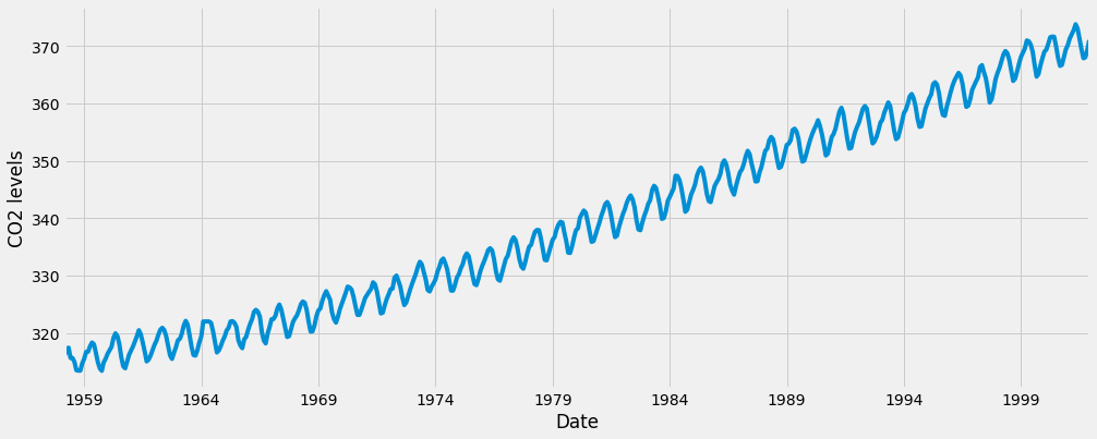
Some distinguishable patterns appear when we plot the data. The time series has an obvious seasonality pattern, as well as an overall increasing trend.
To learn more about time series pre-processing, please refer to “A Guide to Time Series Visualization with Python 3,” where the steps above are described in much more detail.
Now that we’ve converted and explored our data, let’s move on to time series forecasting with ARIMA.
Step 3 — The ARIMA Time Series Model
One of the most common methods used in time series forecasting is known as the ARIMA model, which stands for AutoregRessive Integrated Moving Average. ARIMA is a model that can be fitted to time series data in order to better understand or predict future points in the series.
There are three distinct integers (p, d, q) that are used to parametrize ARIMA models. Because of that, ARIMA models are denoted with the notation ARIMA(p, d, q). Together these three parameters account for seasonality, trend, and noise in datasets:
p is the auto-regressive part of the model. It allows us to incorporate the effect of past values into our model. Intuitively, this would be similar to stating that it is likely to be warm tomorrow if it has been warm the past 3 days.d is the integrated part of the model. This includes terms in the model that incorporate the amount of differencing (i.e. the number of past time points to subtract from the current value) to apply to the time series. Intuitively, this would be similar to stating that it is likely to be same temperature tomorrow if the difference in temperature in the last three days has been very small.q is the moving average part of the model. This allows us to set the error of our model as a linear combination of the error values observed at previous time points in the past.
When dealing with seasonal effects, we make use of the seasonal ARIMA, which is denoted as ARIMA(p,d,q)(P,D,Q)s. Here, (p, d, q) are the non-seasonal parameters described above, while (P, D, Q) follow the same definition but are applied to the seasonal component of the time series. The term s is the periodicity of the time series (4 for quarterly periods, 12 for yearly periods, etc.).
The seasonal ARIMA method can appear daunting because of the multiple tuning parameters involved. In the next section, we will describe how to automate the process of identifying the optimal set of parameters for the seasonal ARIMA time series model.
Step 4 — Parameter Selection for the ARIMA Time Series Model
When looking to fit time series data with a seasonal ARIMA model, our first goal is to find the values of ARIMA(p,d,q)(P,D,Q)s that optimize a metric of interest. There are many guidelines and best practices to achieve this goal, yet the correct parametrization of ARIMA models can be a painstaking manual process that requires domain expertise and time. Other statistical programming languages such as R provide automated ways to solve this issue, but those have yet to be ported over to Python. In this section, we will resolve this issue by writing Python code to programmatically select the optimal parameter values for our ARIMA(p,d,q)(P,D,Q)s time series model.
We will use a “grid search” to iteratively explore different combinations of parameters. For each combination of parameters, we fit a new seasonal ARIMA model with the SARIMAX() function from the statsmodels module and assess its overall quality. Once we have explored the entire landscape of parameters, our optimal set of parameters will be the one that yields the best performance for our criteria of interest. Let’s begin by generating the various combination of parameters that we wish to assess:
p = d = q = range(0, 2)
pdq = list(itertools.product(p, d, q))
seasonal_pdq = [(x[0], x[1], x[2], 12) for x in list(itertools.product(p, d, q))]
print('Examples of parameter combinations for Seasonal ARIMA...')
print('SARIMAX: {} x {}'.format(pdq[1], seasonal_pdq[1]))
print('SARIMAX: {} x {}'.format(pdq[1], seasonal_pdq[2]))
print('SARIMAX: {} x {}'.format(pdq[2], seasonal_pdq[3]))
print('SARIMAX: {} x {}'.format(pdq[2], seasonal_pdq[4]))
Output
Examples of parameter combinations for Seasonal ARIMA...
SARIMAX: (0, 0, 1) x (0, 0, 1, 12)
SARIMAX: (0, 0, 1) x (0, 1, 0, 12)
SARIMAX: (0, 1, 0) x (0, 1, 1, 12)
SARIMAX: (0, 1, 0) x (1, 0, 0, 12)
We can now use the triplets of parameters defined above to automate the process of training and evaluating ARIMA models on different combinations. In Statistics and Machine Learning, this process is known as grid search (or hyperparameter optimization) for model selection.
When evaluating and comparing statistical models fitted with different parameters, each can be ranked against one another based on how well it fits the data or its ability to accurately predict future data points. We will use the AIC (Akaike Information Criterion) value, which is conveniently returned with ARIMA models fitted using statsmodels. The AIC measures how well a model fits the data while taking into account the overall complexity of the model. A model that fits the data very well while using lots of features will be assigned a larger AIC score than a model that uses fewer features to achieve the same goodness-of-fit. Therefore, we are interested in finding the model that yields the lowest AIC value.
The code chunk below iterates through combinations of parameters and uses the SARIMAX function from statsmodels to fit the corresponding Seasonal ARIMA model. Here, the order argument specifies the (p, d, q) parameters, while the seasonal_order argument specifies the (P, D, Q, S) seasonal component of the Seasonal ARIMA model. After fitting each SARIMAX()model, the code prints out its respective AICscore.
warnings.filterwarnings("ignore")
for param in pdq:
for param_seasonal in seasonal_pdq:
try:
mod = sm.tsa.statespace.SARIMAX(y,
order=param,
seasonal_order=param_seasonal,
enforce_stationarity=False,
enforce_invertibility=False)
results = mod.fit()
print('ARIMA{}x{}12 - AIC:{}'.format(param, param_seasonal, results.aic))
except:
continue
Because some parameter combinations may lead to numerical misspecifications, we explicitly disabled warning messages in order to avoid an overload of warning messages. These misspecifications can also lead to errors and throw an exception, so we make sure to catch these exceptions and ignore the parameter combinations that cause these issues.
The code above should yield the following results, this may take some time:
Output
SARIMAX(0, 0, 0)x(0, 0, 1, 12) - AIC:6787.3436240402125
SARIMAX(0, 0, 0)x(0, 1, 1, 12) - AIC:1596.711172764114
SARIMAX(0, 0, 0)x(1, 0, 0, 12) - AIC:1058.9388921320026
SARIMAX(0, 0, 0)x(1, 0, 1, 12) - AIC:1056.2878315690562
SARIMAX(0, 0, 0)x(1, 1, 0, 12) - AIC:1361.6578978064144
SARIMAX(0, 0, 0)x(1, 1, 1, 12) - AIC:1044.7647912940095
...
...
...
SARIMAX(1, 1, 1)x(1, 0, 0, 12) - AIC:576.8647112294245
SARIMAX(1, 1, 1)x(1, 0, 1, 12) - AIC:327.9049123596742
SARIMAX(1, 1, 1)x(1, 1, 0, 12) - AIC:444.12436865161305
SARIMAX(1, 1, 1)x(1, 1, 1, 12) - AIC:277.7801413828764
The output of our code suggests that SARIMAX(1, 1, 1)x(1, 1, 1, 12) yields the lowest AIC value of 277.78. We should therefore consider this to be optimal option out of all the models we have considered.
Step 5 — Fitting an ARIMA Time Series Model
Using grid search, we have identified the set of parameters that produces the best fitting model to our time series data. We can proceed to analyze this particular model in more depth.
We’ll start by plugging the optimal parameter values into a new SARIMAX model:
mod = sm.tsa.statespace.SARIMAX(y,
                                order=(1, 1, 1),
                                seasonal_order=(1, 1, 1, 12),
                                enforce_stationarity=False,
                                enforce_invertibility=False)

results = mod.fit()

print(results.summary().tables[1])
Output
==============================================================================
                 coef    std err          z      P>|z|      [0.025      0.975]
------------------------------------------------------------------------------
ar.L1          0.3182      0.092      3.443      0.001       0.137       0.499
ma.L1         -0.6255      0.077     -8.165      0.000      -0.776      -0.475
ar.S.L12       0.0010      0.001      1.732      0.083      -0.000       0.002
ma.S.L12      -0.8769      0.026    -33.811      0.000      -0.928      -0.826
sigma2         0.0972      0.004     22.634      0.000       0.089       0.106
==============================================================================
The summary attribute that results from the output of SARIMAX returns a significant amount of information, but we’ll focus our attention on the table of coefficients. The coef column shows the weight (i.e. importance) of each feature and how each one impacts the time series. The P>|z| column informs us of the significance of each feature weight. Here, each weight has a p-value lower or close to 0.05, so it is reasonable to retain all of them in our model.
When fitting seasonal ARIMA models (and any other models for that matter), it is important to run model diagnostics to ensure that none of the assumptions made by the model have been violated. The plot_diagnostics object allows us to quickly generate model diagnostics and investigate for any unusual behavior.
results.plot_diagnostics(figsize=(15, 12))
plt.show()
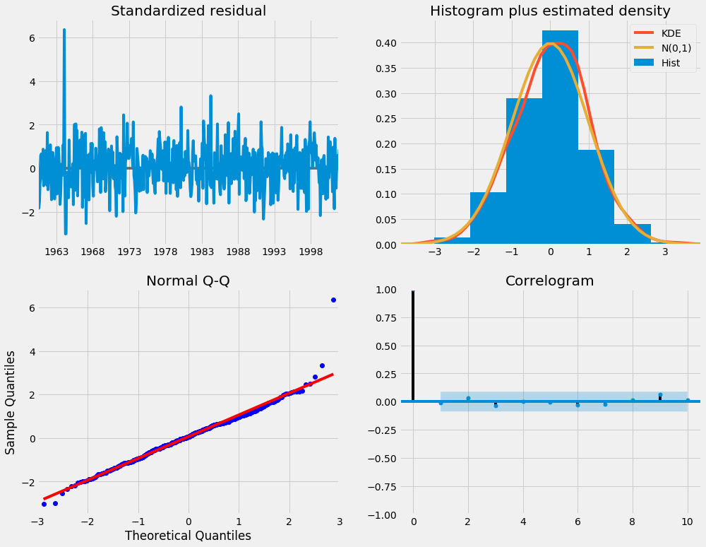
Our primary concern is to ensure that the residuals of our model are uncorrelated and normally distributed with zero-mean. If the seasonal ARIMA model does not satisfy these properties, it is a good indication that it can be further improved.
In this case, our model diagnostics suggests that the model residuals are normally distributed based on the following:
- In the top right plot, we see that the red
KDE line follows closely with the N(0,1) line (where N(0,1)) is the standard notation for a normal distribution with mean 0 and standard deviation of 1). This is a good indication that the residuals are normally distributed.
- The qq-plot on the bottom left shows that the ordered distribution of residuals (blue dots) follows the linear trend of the samples taken from a standard normal distribution with
N(0, 1). Again, this is a strong indication that the residuals are normally distributed.
- The residuals over time (top left plot) don’t display any obvious seasonality and appear to be white noise. This is confirmed by the autocorrelation (i.e. correlogram) plot on the bottom right, which shows that the time series residuals have low correlation with lagged versions of itself.
Those observations lead us to conclude that our model produces a satisfactory fit that could help us understand our time series data and forecast future values.
Although we have a satisfactory fit, some parameters of our seasonal ARIMA model could be changed to improve our model fit. For example, our grid search only considered a restricted set of parameter combinations, so we may find better models if we widened the grid search.
Step 6 — Validating Forecasts
We have obtained a model for our time series that can now be used to produce forecasts. We start by comparing predicted values to real values of the time series, which will help us understand the accuracy of our forecasts. The get_prediction() and conf_int() attributes allow us to obtain the values and associated confidence intervals for forecasts of the time series.
pred = results.get_prediction(start=pd.to_datetime('1998-01-01'), dynamic=False)
pred_ci = pred.conf_int()
The code above requires the forecasts to start at January 1998.
The dynamic=False argument ensures that we produce one-step ahead forecasts, meaning that forecasts at each point are generated using the full history up to that point.
We can plot the real and forecasted values of the CO2 time series to assess how well we did. Notice how we zoomed in on the end of the time series by slicing the date index.
ax = y['1990':].plot(label='observed')
pred.predicted_mean.plot(ax=ax, label='One-step ahead Forecast', alpha=.7)

ax.fill_between(pred_ci.index,
                pred_ci.iloc[:, 0],
                pred_ci.iloc[:, 1], color='k', alpha=.2)

ax.set_xlabel('Date')
ax.set_ylabel('CO2 Levels')
plt.legend()

plt.show()
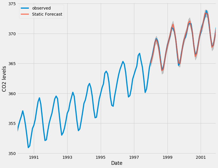
Overall, our forecasts align with the true values very well, showing an overall increase trend.
It is also useful to quantify the accuracy of our forecasts. We will use the MSE (Mean Squared Error), which summarizes the average error of our forecasts. For each predicted value, we compute its distance to the true value and square the result. The results need to be squared so that positive/negative differences do not cancel each other out when we compute the overall mean.
y_forecasted = pred.predicted_mean
y_truth = y['1998-01-01':]
mse = ((y_forecasted - y_truth) ** 2).mean()
print('The Mean Squared Error of our forecasts is {}'.format(round(mse, 2)))
Output
The Mean Squared Error of our forecasts is 0.07
The MSE of our one-step ahead forecasts yields a value of 0.07, which is very low as it is close to 0. An MSE of 0 would that the estimator is predicting observations of the parameter with perfect accuracy, which would be an ideal scenario but it not typically possible.
However, a better representation of our true predictive power can be obtained using dynamic forecasts. In this case, we only use information from the time series up to a certain point, and after that, forecasts are generated using values from previous forecasted time points.
In the code chunk below, we specify to start computing the dynamic forecasts and confidence intervals from January 1998 onwards.
pred_dynamic = results.get_prediction(start=pd.to_datetime('1998-01-01'), dynamic=True, full_results=True)
pred_dynamic_ci = pred_dynamic.conf_int()
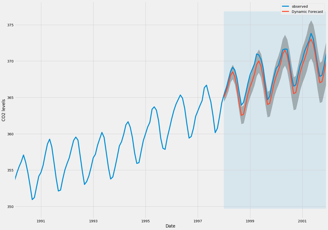
Plotting the observed and forecasted values of the time series, we see that the overall forecasts are accurate even when using dynamic forecasts. All forecasted values (red line) match pretty closely to the ground truth (blue line), and are well within the confidence intervals of our forecast.
ax = y['1990':].plot(label='observed', figsize=(20, 15))
pred_dynamic.predicted_mean.plot(label='Dynamic Forecast', ax=ax)

ax.fill_between(pred_dynamic_ci.index,
                pred_dynamic_ci.iloc[:, 0],
                pred_dynamic_ci.iloc[:, 1], color='k', alpha=.25)

ax.fill_betweenx(ax.get_ylim(), pd.to_datetime('1998-01-01'), y.index[-1],
                 alpha=.1, zorder=-1)

ax.set_xlabel('Date')
ax.set_ylabel('CO2 Levels')

plt.legend()
plt.show()
Once again, we quantify the predictive performance of our forecasts by computing the MSE:
y_forecasted = pred_dynamic.predicted_mean
y_truth = y['1998-01-01':]
mse = ((y_forecasted - y_truth) ** 2).mean()
print('The Mean Squared Error of our forecasts is {}'.format(round(mse, 2)))
Output
The Mean Squared Error of our forecasts is 1.01
The predicted values obtained from the dynamic forecasts yield an MSE of 1.01. This is slightly higher than the one-step ahead, which is to be expected given that we are relying on less historical data from the time series.
Both the one-step ahead and dynamic forecasts confirm that this time series model is valid. However, much of the interest around time series forecasting is the ability to forecast future values way ahead in time.
Step 7 — Producing and Visualizing Forecasts
In the final step of this tutorial, we describe how to leverage our seasonal ARIMA time series model to forecast future values. The get_forecast() attribute of our time series object can compute forecasted values for a specified number of steps ahead.
pred_uc = results.get_forecast(steps=500)
pred_ci = pred_uc.conf_int()
We can use the output of this code to plot the time series and forecasts of its future values.
ax = y.plot(label='observed', figsize=(20, 15))
pred_uc.predicted_mean.plot(ax=ax, label='Forecast')
ax.fill_between(pred_ci.index,
                pred_ci.iloc[:, 0],
                pred_ci.iloc[:, 1], color='k', alpha=.25)
ax.set_xlabel('Date')
ax.set_ylabel('CO2 Levels')

plt.legend()
plt.show()
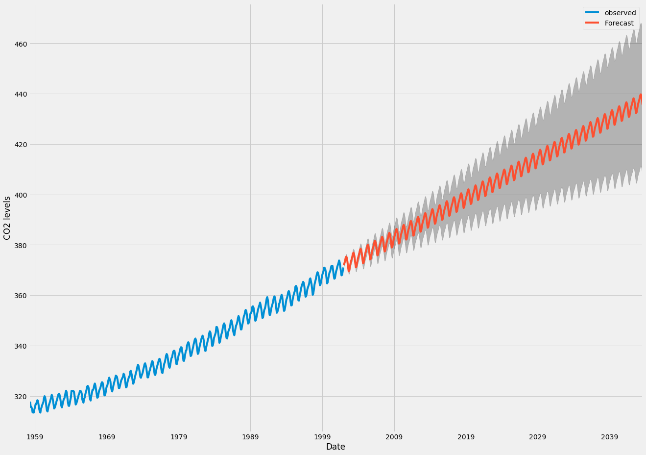
Both the forecasts and associated confidence interval that we have generated can now be used to further understand the time series and foresee what to expect. Our forecasts show that the time series is expected to continue increasing at a steady pace.
As we forecast further out into the future, it is natural for us to become less confident in our values. This is reflected by the confidence intervals generated by our model, which grow larger as we move further out into the future.
Conclusion
In this tutorial, we described how to implement a seasonal ARIMA model in Python. We made extensive use of the pandas and statsmodels libraries and showed how to run model diagnostics, as well as how to produce forecasts of the CO2 time series.
Here are a few other things you could try:
- Change the start date of your dynamic forecasts to see how this affects the overall quality of your forecasts.
- Try more combinations of parameters to see if you can improve the goodness-of-fit of your model.
- Select a different metric to select the best model. For example, we used the
AIC measure to find the best model, but you could seek to optimize the out-of-sample mean square error instead.
For more practice, you could also try to load another time series dataset to produce your own forecasts.


 本,那么一本一本检测的话需要
  次;当
次;当  很大的时候,可以清楚地知道
  ,其检测的次数会呈现明显的减少。
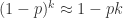
 )。令 p = m / n 表示患病率且 p < 0.01。为了减少检测量,检测人员想对人群进行分桶操作,每 k 个人的样本进行混合,并且对这个混合样本进行检测。如果该混合样本没有问题,则这 k 个人都没有问题;如果该混合样本有问题,则再次对这 k 个人进行逐一检测。通过这样的方法,就可以得到最终的结果。那么,这个 k 该如何选择呢?
 ,有问题的概率是
  。那么,这 k 个人总检测次数的期望值就是
  。由于城市 A 总共有 n 个人,那么就需要 n / k 个桶,因此,总检测次数的期望是
  。
。 ,因此,总检测次数的期望值约等于
  。当
。当 时,上述公式达到最小值
  。如果 p=0.01 时,k 取 10 可以达到最小值
  ;当 p=0.001 时,k 取 32 可以达到最小值
  。通过混合采样的方法,可以将总检测次数的期望变成原来的五分之一甚至十分之一以下。
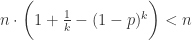 ,化简之后得到
 ![p<1-\frac{1}{\sqrt[k]{k}}](https://s0.wp.com/latex.php?latex=p%3C1-%5Cfrac%7B1%7D%7B%5Csqrt%5Bk%5D%7Bk%7D%7D&bg=ffffff&fg=2b2b2b&s=0&c=20201002) 。
。 其中
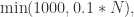
其中  表示总量;例如,当
  时,最大样本数可以选择 500;而当
  时,最大样本数只需要选择 1000 即可;


 表示总体中满足某个选项的数量,
 表示样本中满足某个选项的数量。令

 ,且正态分布的概率用 Prob 表示,那么
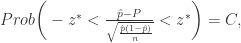
 . 其中
. 其中  和
和 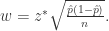

 所以,
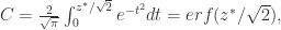
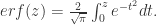
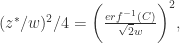
所以, 最大样本数可以选择为

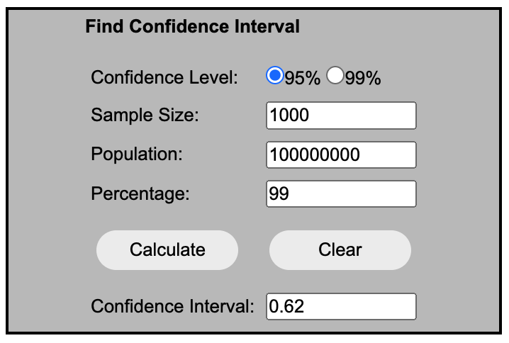
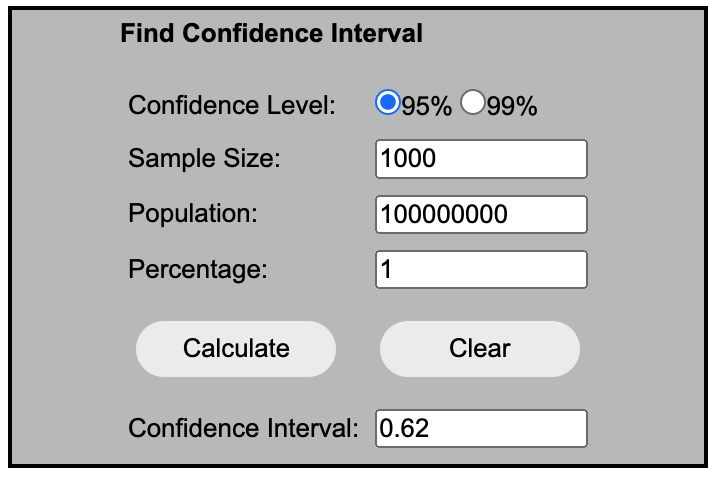
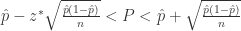
 表示置信区间,
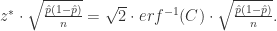

 置信度
置信度  的时候,最大样本数是:
 的时候,最大样本数是:


 置信区间是
置信区间是 


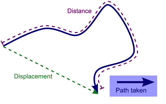
 和
和  之间的距离,通常可以使用
  范数来进行描述,其数学公式是:


 并且满足以下条件:
 对于所有的
对于所有的  都成立;
都成立;
 对于所有的
对于所有的  对于所有的
对于所有的  都成立。
都成立。 指的是在其定义域内的任意两个点
  满足
满足 换言之,如果凸函数
  存在二阶连续导数,那么
  是增函数,
是增函数,
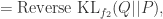
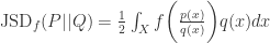
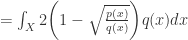
 来定义两个概率分布之间的距离。该函数
  是一个凸函数(convex function),并且满足
  对于空间
对于空间  和
和  而言,
而言,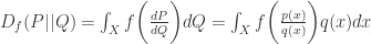
 散度(f-divergence),其中
  分别对应了
分别对应了  的概率密度函数。不同的函数
 或者
或者 

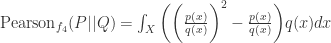
 – 散度(Pearson
  或者
或者  或者
或者 
 或者
或者 


 是非负函数,i.e.
  事实上,
事实上,
 在定义域
在定义域  也是凸函数。
 有
有
 时,其距离公式是:


 分别对应着 KL-散度和 Reverse KL-散度相应函数的原因。
 和
和 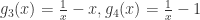 而言,可以直接证明得到:


 i.e.
i.e. 
 其实这两个函数是等价的,因为


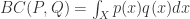 被称为 Bhattacharyya 系数(Bhattacharyya Coefficient),Bhattacharyya 距离则定义为
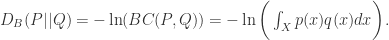
 因此当
因此当  时,
时,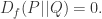

 所以可以得到
 同时,Bhattacharyya 距离
  是没有上界的,因为
  可以取值到零。
 并且上界 2 是可以取到的。


 时,
时, 可以看成集合,也可以看成重数为 1 的多重集合,可以记为
  或者
或者 
 中,
中, 的重数是 2,
 的重数是 1,可以记为
  或者
或者 
 中,
中, 的重数都是 3。
 而言,其多重集合可以记为
  或者
或者  其中
其中  表示元素
表示元素  的重数。多重集合的一个典型例子就是质因数分解,例如:
 的元素都属于集合
 有
有  则称多重集合
  是多重集合
是多重集合  的子集;
的子集; 则称多重集合
 则称多重集合
 则称多重集合
 则称多重集合
 那么
那么


 而言,令
而言,令  因此,多重集合
  于是,可以使用以上的统计距离(Statistical Distance)来计算两个多重集合之间的距离。


![G_{n}=\sqrt[n]{x_{1}\cdots x_{n}}.](https://s0.wp.com/latex.php?latex=G_%7Bn%7D%3D%5Csqrt%5Bn%5D%7Bx_%7B1%7D%5Ccdots+x_%7Bn%7D%7D.&bg=ffffff&fg=2b2b2b&s=0&c=20201002)


 都是正数,那么
  也就是说,调和平均数
 几何平均数
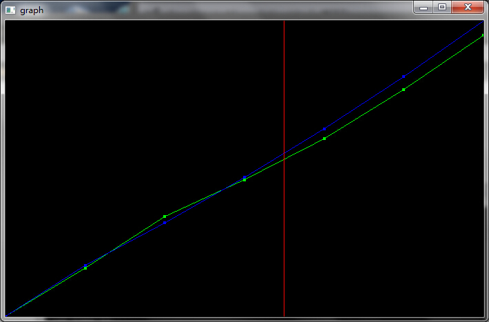
几何平均数 的情形证明如下图。其余可以用数学归纳法等多种方法证明。
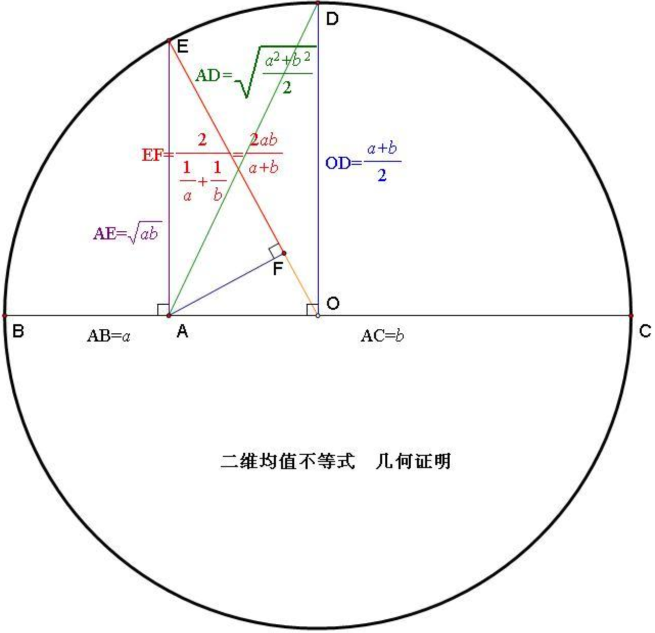
 而标准差则有两种情况,第一种是总体的样本差(population standard deviation),总体的标准差定义为方差正的平方根,记为 SD,

 是从一个更大的总体抽样出来的部分数据。样本的标准差记为
 的定义为
的定义为
 阶矩指的是
阶矩指的是
 就是算术平均数。
 就是样本方差。
 其中
其中 
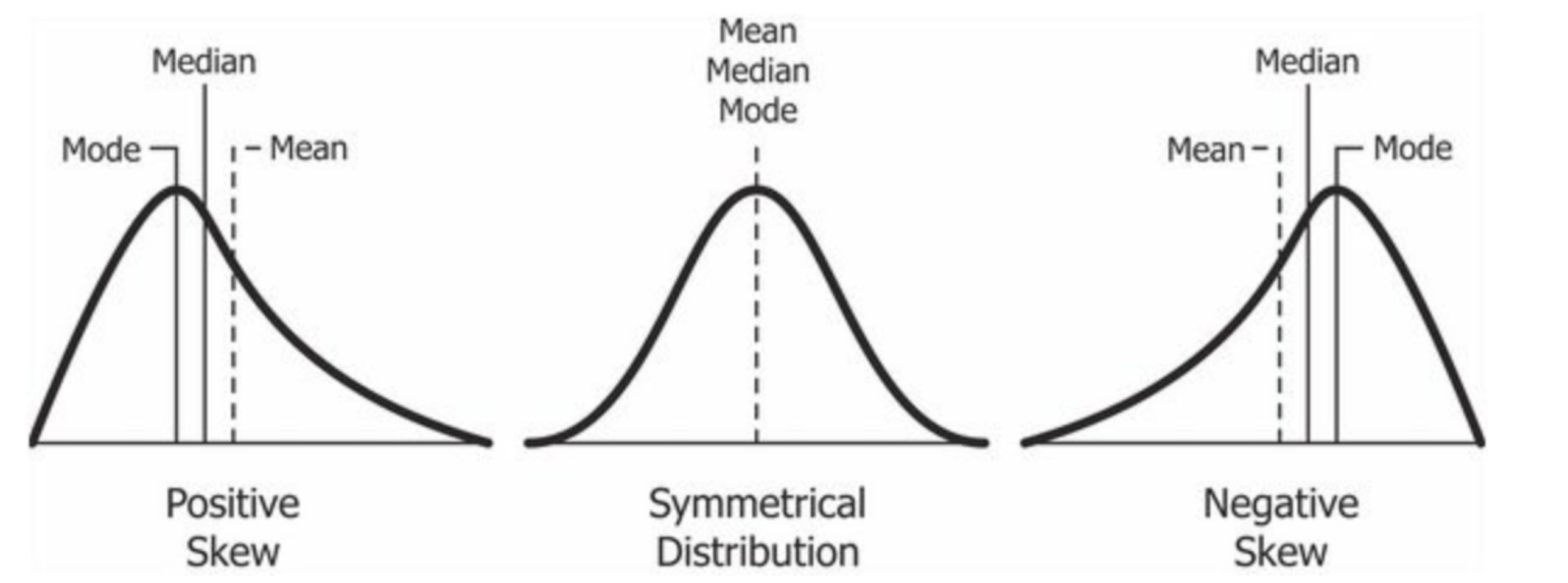
 而偏度的结果可以是正数,负数,或者零。分别被称为 Positive Skew(右侧的尾巴更长), Negative Skew(左侧的尾巴更长) 和 Zero Skew。当均值等于中位数等于众数的时候,该概率分布是对称的。Median(中位数)相对于 Mean(均值)是更加接近 Mode(众数)的数字,因此根据 Median 和 Mean 的大小关系也能够大致判断 Skew(偏度)的趋势。
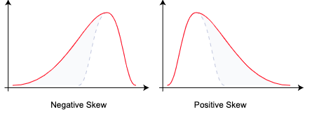
 其中
其中 
 减去 3 的目的是为了让正态分布的峰度为零。
 的值。可以使用极坐标的方法来解决,首先通过坐标变换可以得到原式子等于
  其次,令
其次,令  可以得到
可以得到


 从而原式子等于 3。i.e. 正态分布 4 阶距的值是 3。
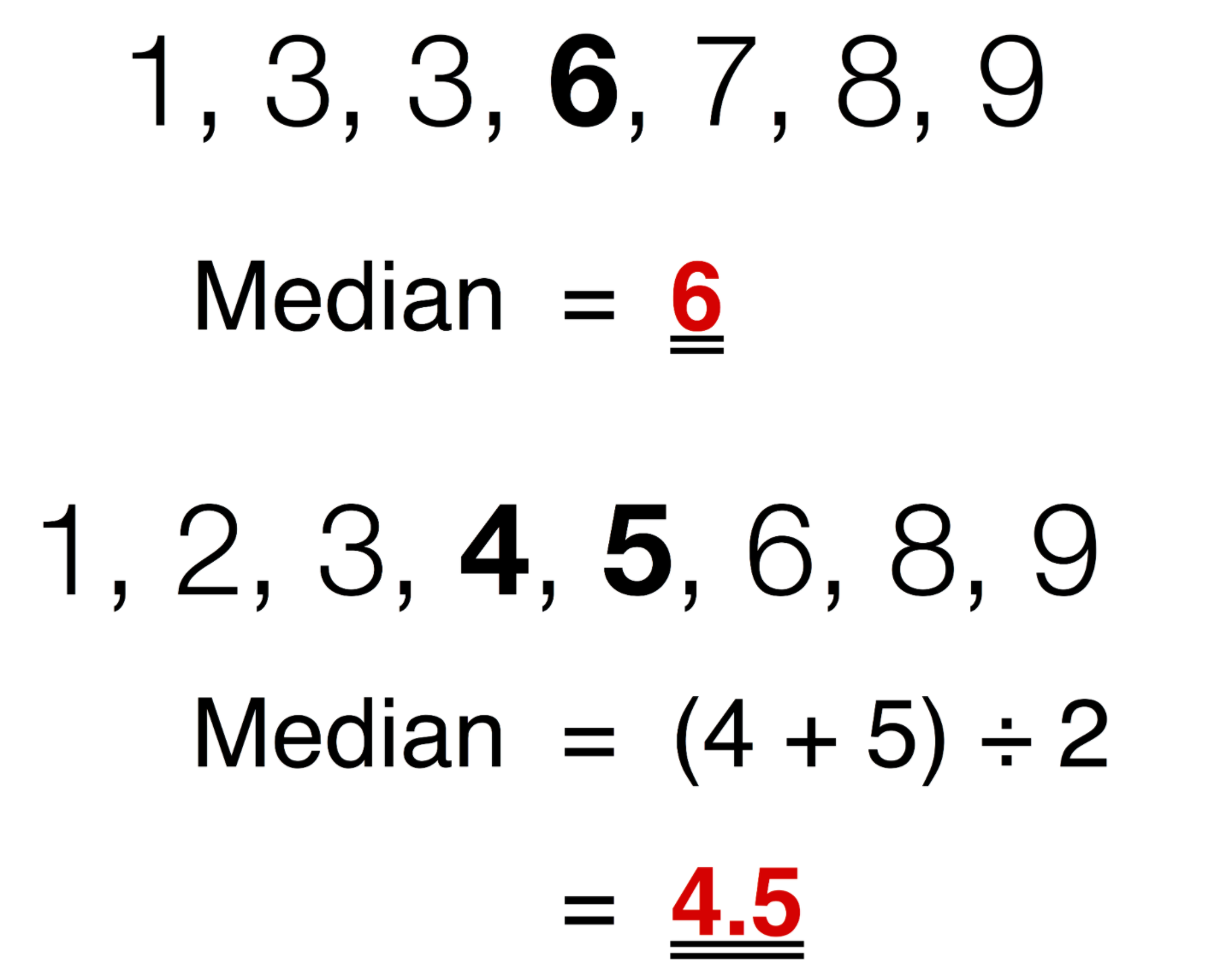
 可以设置其一组正数权重
  然后得到其带权重的算术平均数为
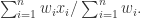
 的数列而言,
 就是
就是  就是
就是 


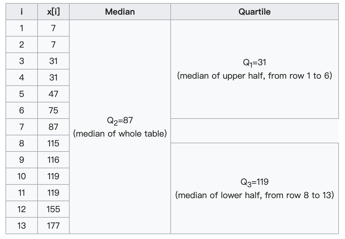
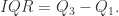
 从而四分位距
  异常检测的上下界分别是

 和
和  两个集合。对于
  它的
它的  四分位发散系数为
  对于
对于  而言,
而言, 它的
它的  ,四分位发散系数为
  因此集合
因此集合 
 而言,平均绝对偏差(Mean Absolute Difference)定义为:

 其中
其中  可以看出数据的偏移程度。
 通过定义可以计算出它们的变异系数
  变异系数越大,表示集合的数据波动程度越大。变异系数越小,表示集合的数据波动程度越小。
 是全集
是全集 则是集合
则是集合
 ,这个方法的时间复杂度是指数级别的。


 到
到


 ,
, 
 。这样该模型的错误率就是


 当训练集并且


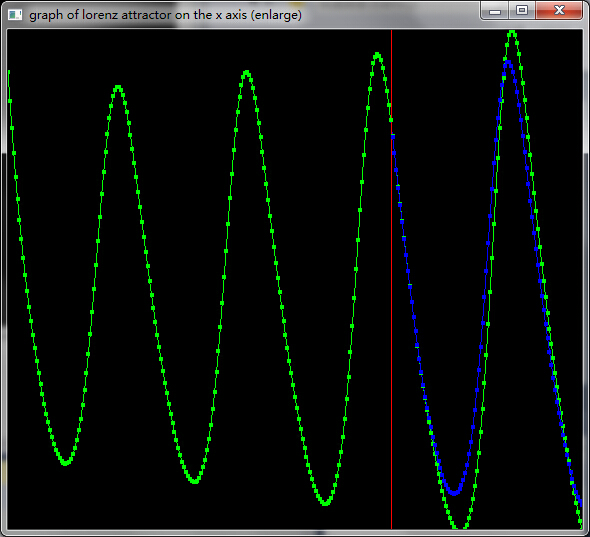
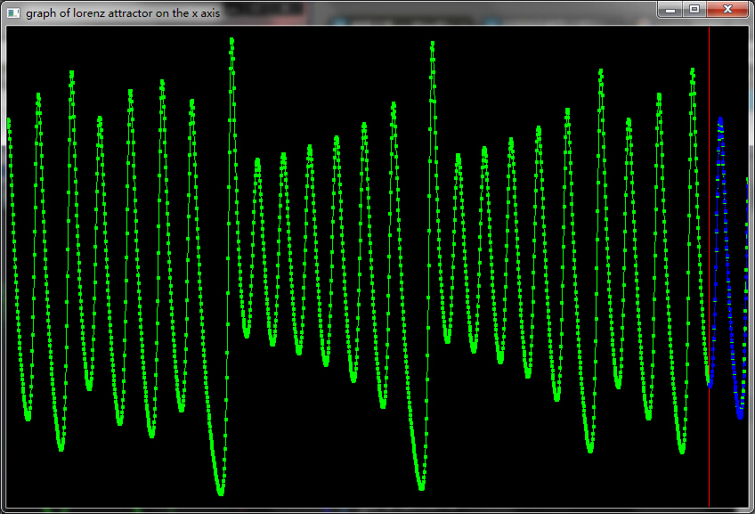
 那么吸引子的结构特性就包含在这个时间序列之中。为了从时间序列中提取出更多有用的信息,1980年Packard等人提出了时间序列重构相空间的两种方法:导数重构法和坐标延迟重构法。而后者的本质则是通过一维的时间序列
 的不同延迟时间
 来构建
来构建 维的相空间矢量
 维混沌吸引子的一维标量时间序列
 都可以在拓扑不变的意义下找到一个
 根据Takens嵌入定理,我们可以从一维混沌时间序列中重构一个与原动力系统在拓扑意义下一样的相空间,混沌时间序列的判定,分析和预测都是在这个重构的相空间中进行的,因此相空间的重构就是混沌时间序列研究的关键。
 在Takens嵌入定理中,嵌入维数和延迟时间都只是理论上证明了其存在性,并没有给出具体的表达式,而且实际应用中时间序列都是有噪声的有限序列,嵌入维数和时间延迟必须要根据实际的情况来选取合适的值。
 与
与 在数值上非常接近,以至于无法相互区分,从而无法提供两个独立的坐标分量;但是如果延迟时间
 从而在独立和相关两者之间达到一种平衡。
 可以写出其自相关函数如下:
 来做出自相关函数
 随着延迟时间
 的
的 时,i.e.
  所得到的时间
 以及
以及 之间不相关,但是
 之间的相关性可能会很强。这一点意味着这种方法并不能够有效的推广到高维的研究。而且选择下降系数
 所构成的系统
 和
和

 分别是
分别是 和
和 的概率。交互信息的计算公式是:

 称为事件
称为事件 的联合分布概率。交互信息标准化就是
 也就是
也就是
 那么
那么 则是关于延迟时间
 的大小表示在已知系统
 的情况下,系统
 的确定性的大小。
 表示
表示 和
和 这里采取的方法是等间距格子法,其方法简要概述如下。
 在
在 平面用一个矩形包含上面所有的点。将矩形
 份,
份, 份(注:
份(注: 取值100~200之间即可)。那么在
 假设
假设 是
是 那么
那么![Row[i]](https://s0.wp.com/latex.php?latex=Row%5Bi%5D&bg=ffffff&fg=2b2b2b&s=0&c=20201002) 做一次记录;
做一次记录; 那么
那么 在第
在第 个格子中,对
![Col[j]](https://s0.wp.com/latex.php?latex=Col%5Bj%5D&bg=ffffff&fg=2b2b2b&s=0&c=20201002) 做一次记录。
做一次记录。 那么
那么![P_{S}(i)=Row[i]/(n-\tau), 1\leq i\leq M_{1},](https://s0.wp.com/latex.php?latex=P_%7BS%7D%28i%29%3DRow%5Bi%5D%2F%28n-%5Ctau%29%2C+1%5Cleq+i%5Cleq+M_%7B1%7D%2C&bg=ffffff&fg=2b2b2b&s=0&c=20201002)
![P_{Q}(j)=Col[j]/(n-\tau), 1\leq j\leq M_{2}.](https://s0.wp.com/latex.php?latex=P_%7BQ%7D%28j%29%3DCol%5Bj%5D%2F%28n-%5Ctau%29%2C+1%5Cleq+j%5Cleq+M_%7B2%7D.&bg=ffffff&fg=2b2b2b&s=0&c=20201002)
 且
且 则
则 在标号为
在标号为 的格子中,对
![Together[i][j]](https://s0.wp.com/latex.php?latex=Together%5Bi%5D%5Bj%5D&bg=ffffff&fg=2b2b2b&s=0&c=20201002) 做一次记录。那么
做一次记录。那么![P_{S,Q}(i,j)=Together[i][j]/(n-\tau)^{2}, 1\leq i\leq M_{1}, 1\leq j\leq M_{2}.](https://s0.wp.com/latex.php?latex=P_%7BS%2CQ%7D%28i%2Cj%29%3DTogether%5Bi%5D%5Bj%5D%2F%28n-%5Ctau%29%5E%7B2%7D%2C+1%5Cleq+i%5Cleq+M_%7B1%7D%2C+1%5Cleq+j%5Cleq+M_%7B2%7D.&bg=ffffff&fg=2b2b2b&s=0&c=20201002)


 第一次下降到极小值所对应的延迟时间
 实际应用中通常的方法是计算吸引子的某些几何不变量(如关联维数,Lyapunov指数等)。选择好延迟时间
 其距离是
其距离是
 时,这两个点的距离就会发生变化,新的距离是
 并且
并且
 比
比 大很多,那么就可以认为这是由于高维混沌吸引子中两个不相邻得点投影到低维坐标上变成相邻的两点造成的,这样的临近点是虚假的,令
![a_{1}(i,d)>R_{\tau} \in [10,50],](https://s0.wp.com/latex.php?latex=a_%7B1%7D%28i%2Cd%29%3ER_%7B%5Ctau%7D+%5Cin+%5B10%2C50%5D%2C&bg=ffffff&fg=2b2b2b&s=0&c=20201002) 那么
那么 就是
就是 的虚假最临近点。这里的
 是阀值。
是阀值。 具有很强的主观性。此时Cao Liangyue教授提出了改进的FNN方法,此方法计算时只需要延迟时间
 那么基于延迟时间
 这里的
这里的
 是最大模范数。其中
 是第
是第
 是使得
是使得 ,显然
,显然 由
由
 与延迟时间
与延迟时间 当
当 时,
时, 不再变化,那么
 则是我们所寻找的最小嵌入维数。除了
 还可以定义一个变量
 如下。令
如下。令
 定义
定义 对于随机序列,数据之间没有相关性,
 对于确定性的序列,数据点之间的关系依赖于嵌入维数
 可以确定其延迟时间
 个
个


 建立一个动力系统的模型如下:
 其中
其中 是一个连续函数。
 根据连续函数的性质可以知道:如果
 与
与 非常接近,那么
 与
与 也是非常接近的,可以用
 作为
作为 的近似值。
的近似值。 i.e. 也就是从其他的
 个向量中选取前
 或者最大模范数
 根据局部预测法的观点,可以得到
 的近似值:
的近似值:


 是待定系数。假设向量
 此处可以用欧几里德范数
 使得
使得


 矩阵
矩阵 根据最小二乘法可以得到待定系数向量
 是最小二乘解。


 是系统的三个坐标,
 是三个系数。在这里,我们取
 在解这个常微分方程的时候,使用了经典的Runge-Kutta数值方法。
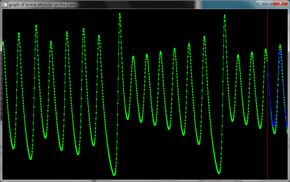


 ,其中n是数组的长度。通过分析这组序列的内在结构,从而建立相应的微分方程模型,达到预测未来序列
 的目的。
的目的。 ,其中
,其中


 , 它的离散方程是
 这里
这里 其中a成为发展系数,b称为控制系数。通过最小二乘法的推导,可以得到
  其中B和Y都是矩阵,定义如下:
 ,
,

 从而得到序列的预测值:


 从而得到的序列的预测值:
 离散方程则是
 通过最小二乘法的推导,可以得到
  ,
, 从而可以得到预测的序列

 , 那么
, 那么
 通过最小二乘法的推导,可以得到
  ,
,


 通过计算累积生成序列,可以进一步求的系数a和b的值,从而根据上面的模型进行模拟。通过模型可以算出


 通过计算累积生成序列,可以进一步求的系数a和b的值,从而根据上面的模型进行模拟。通过模型可以算出


9 Comments