Reference Book: Joel L.Schiff- Normal Families
Some Classical Theorems
Weierstrass Theorem Let  be a sequence of analytic functions on a domain
  which converges uniformly on compact subsets of to a function
  . Then is analytic in , and the sequence of derivatives
  converges uniformly on compact subsets to
  .
.
Hurwitz Theorem Let be a sequence of analytic functions on a domain which converges uniformly on compact subsets of to a non-constant analytic function  . If
. If  for some
  , then for each
  sufficiently small, there exists an
  , such that for all
  ,
,  has the same number of zeros in
  as does . (The zeros are counted according to multiplicity).
The Maximum Principle If is analytic and non-constant in a region , then its absolute value  has no maximum in .
The Maximum Principle’ If is defined and continuous on a closed bounded set  and analytic on the interior of , then the maximum of on is assumed on the boundary of .
Corollary 1.4.1 If is a sequence of univalent analytic functions in a domain which converge uniformly on compact subsets of to a non-constant analytic function , then is univalent in .
Definition 1.5.1 A family of functions  is locally bounded on a domain if, for each
  , there is a positive number
  and a neighbourhood
  such that
  for all
  and all
  .
.
Theorem 1.5.2 If is a family of locally bounded analytic functions on a domain , then the family of derivatives  form a locally bounded family in .
The converse of Theorem 1.5.2 is false, since  . However, the following partial converse does hold.
Theorem 1.5.3 Let be a family of analytic functions on such that the family of derivatives  is locally bounded and suppose that there is some with
  for all . Then is locally bounded. (Hint: find a path connecting
  and
and  .)
.)
Definition 1.6.1 A family of functions defined on a domain is said to be equicontinuous (spherically continuous) at a point  if, for each
  , there is a
  such that
  ,
,  whenever
  , for every . Moreover, is equicontinuous (spherical continuous) on a subset
  if it is continuous (spherically continuous) at each point of .
Normal Families of Analytic Functions
Definition 2.1.1 A familiy of analytic functions on a domain  is normal in if every sequence of functions
  contains either a subsequence which converges to a limit function
  uniformly on each compact subset of , or a subsequence which converges uniformly to
  on each compact subset.
The family is said to be normal at a point if it is normal in some neighbourhood of .
Theorem 2.1.2 A family of analytic functions is normal in a domain if and only if is normal at each point in .
Theorem 2.2.1 Arzela-Ascoli Theorem. If a sequence  of continuous functions converges uniformly on a compact set
  to a limit function , then is equicontinuous on , and is continuous. Conversely, if is equicontinuous and locally bounded on , then a subsequence can be extracted from which converges locally uniformly in to a (continuous) limit function .
Montel’s Theorem If is a locally bounded family of analytic functions on a domain , then is a normal family in .
Koebe Distortion Theorem Let be analytic univalent in a domain and a compact subset of . Then there exists a constant  such that for any
  ,
,  .
.
Vitali-Porter Theorem Let be a locally bounded sequence of analytic functions in a domain such that  exists for each belonging to a set which has an accumulation point in . Then converges uniformly on compact subsets of to an analytic function.
Proof. From Montel’s Theorem, is normal, extract a subsequence  which converges normally to an analytic function . Then
  for each
  . Suppose, however, that does not converge uniformly on compact subsets of to . Then there exists some , a compact subset
  , as well as a subsequence
  and points
  satisfying
 . Now
. Now  itself has a subsequence which converges uniformly on compact subsets to an analytic function
  , and
, and  from above. However, since and must agree at all points of , the Identity Theorem for analytic functions implies
  on , a contradiction which establishes the theorem.
Fundamental Normality Test Let be the family of analytic functions on a domain which omit two fixed values  and
and  in
in  . Then is normal in .
Generalized Normality Test Suppose that is a family of analytic functions in a domain which omit a value  and such that no function of assumes the value
  at more that
  points. Then is normal in .
2.3 Examples:
Assume  is the unit disk in the complex plane, is a region (connected open set) in .
1.  in . Then is normal in , but not compact since
  . In the domain
  , is normal.
2.  is a normal family in
  but not compact.
3.  analytic in and
  . Then is normal in and compact.
4. analytic in and  . Then is normal but not compact. Hint:
  is a uniformly bounded family.
5.  analytic, univalent in ,
  . These are the normalised “Schlicht” functions in .
  is normal and compact.
Normal Families of Meromorphic Functions
Assume a function is analytic in a neighbourhood of , except perhaps at itself. In other words, shall be analytic in a region  . The point is called an isolated singularity of . There are three cases about an isolated singularity. The first one is a removable singularity, the second one is a pole, the third one is an essential singularity. A function which is analytic in a region , except for poles, is said to be meromorphic in .
The chordal distance  between
  and
and  is
is
 if and are in the finite plane, and
 if
if  . Clearly,
  , and
, and  . The chordal metric and spherical metric are uniformly equivalent and generate the same open sets on the Riemann sphere.
Definition 1.2.1 A sequence of functions converges spherically uniformly to on a set  if, for any , there is a number
  such that
  implies
  , for all .
Definition 3.1.1 A family of meromorphic functions in a domain is normal in if every sequence  contains a subsequence which converges spherically uniformly on compact subsets of .
Theorem 3.1.3 Let be a sequence of meromorphic functions on a domain . Then converges spherically uniformly on compact subsets of to if and only if about each point there is a closed disk  in which
  or
or  uniformly as
  .
.
Corollary 3.1.4 Let be a sequence of meromorphic functions on which converges spherically uniformly on compact subsets to . Then is either a meromorphic function on or identically equal to .
Corollary 3.1.5 Let be a sequence of analytic functions on a domain which converge spherically uniformly on compact subsets of to . Then is either analytic on or identically equal to .
Theorem 3.2.1 A family of meromorphic functions in a domain is normal if and only if is spherically equicontinuous in .
Fundamental Normality Test Let be a family of meromorphic functions on a domain which omit three distinct values  . Then is normal in .
Vitali-Porter Theorem Let be a sequence belonging to a spherically equicontinuous family of meromorphic functions such that  converges spherically on a point set having an accumulation point in . Then converges spherically uniformly on compact subsets of .
Let be meromorphic on a domain . If  is not a pole, the derivative in the spherical metric, called the spherical derivative, is given by
  . If
. If  is a pole of , define
  .
.
Marty’s Theorem A family of meromorphic functions on a domain is normal if and only if for each compact subset , there exists a constant  such that spherical derivative
  that is,
  is locally bounded.


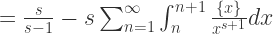
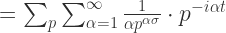
 根据级数与定积分的等价关系可以得到:
 时,
时,
 时,
时,
 上延拓到
上延拓到  上;
上; 上没有零点。
 上,就需要给出 Riemann Zeta 函数在
  上面,新的函数的取值必须与原函数的取值保持一致。
 .
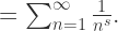
. 时,上述等式显然成立,两侧都是


 可以延拓到
可以延拓到  上。而且右侧的函数在
  是解析的,并且
  的解析函数,而且
  综上所述:
综上所述: 上是解析的;
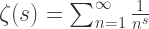
 上。因此,数学家首先要找出的就是 Riemann Zeta 函数的非零区域。而本篇文章将会证明 Riemann Zeta 函数在
  上面没有零点。
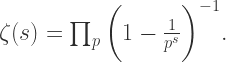
 区域
区域

 表示第
表示第  个素数。
个素数。
 ,当
,当  时,我们有
时,我们有


 when
when 

 直线
直线


 而对于其余的

 可以得到
可以得到


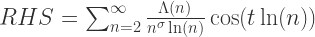


 换句话说
换句话说


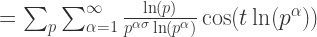
 可以得到
可以得到

 对于所有的
对于所有的  成立。
成立。 存在阶数为
存在阶数为  的零点。也就是说:
 其中
其中 
 并且
并且 


 可以得到左侧趋近于一个有限的值,但是右侧趋近于无穷,所以得到矛盾。也就是说当
  时,
时,  是
是  附近一个“狭长”的区域上,Riemann Zeta 函数没有零点。
 is the unit disc on the complex plane
 is the upper half plane on the complex plane,
 is the band between
  and
and  .
. is defined as
 for all
 is a conformal mapping, where
  , then we can also define the hyperbolic metric on the domain U,
 for all
 is a conformal mapping which maps the upper half plane
  onto the unit disc
  From above formula, we can calculate the hyperbolic metric on
  for all
 is
is for all
 , if the interval
  , then the restriction of the hyperbolic metric on the unit disc
  for all
 . Since there exists a linear map
  which maps a to -1 and b to 1, i.e.
  . Its derivative is
  . Therefore, the hyperbolic metric on the interval I is
 for all
 , then the hyperbolic distance between c and d is

 . Therefore, the hyperbolic distance between c and d in the interval (a,b) equals to

 be a
be a  positive function on an open subset
  is given by
 is the Laplacian operator


 is a conformal mapping, where
  for all
 is
is  .
. , the sphere metric on
  for all
