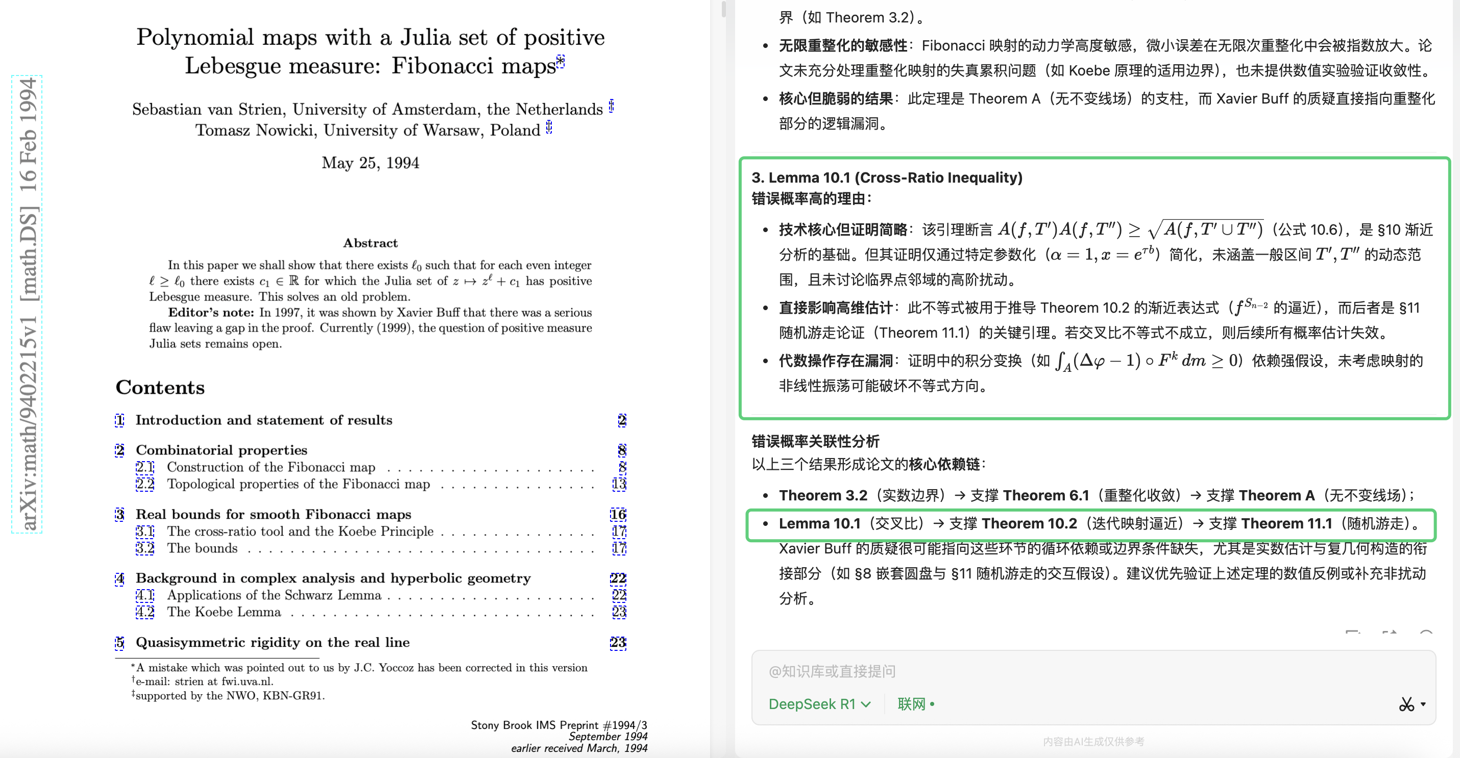
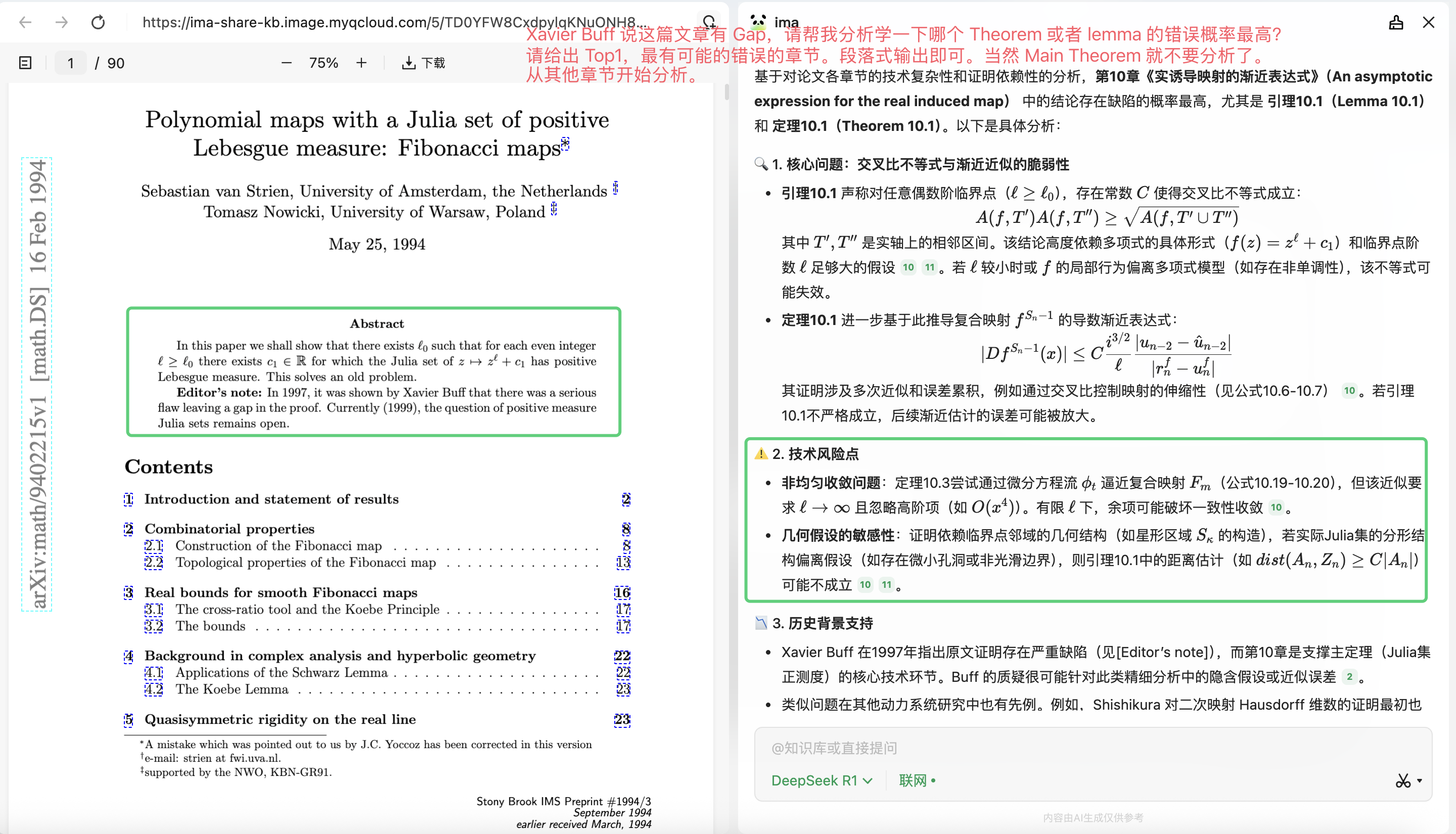
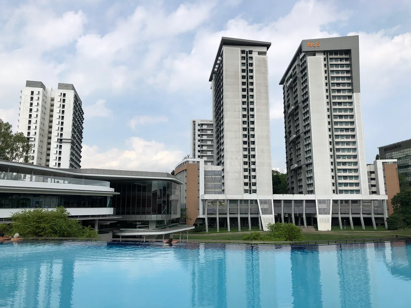
在2010年12月的新加坡,没有冬天,只有雨天。每天差不多下午四点,天色微暗,图书馆的窗外就会下起一场雷阵雨,雷声轰鸣却不让人害怕,反而像是某种自然的节奏。而且下雨的时间非常准时,不多不少,正好是每天下午的四点左右。当年由于办公位紧张,再加上我的运气一般,导致我没有抽到办公位,所以我每天就喜欢坐在新加坡国立大学的理学院图书馆(Science)靠窗的位置,桌上摊着一篇数学论文,题目看起来很有难度:《Polynomial maps with a Julia set of positive Lebesgue measure: Fibonacci maps》。这是导师布置的任务,要我找出这篇论文中的一个“gap”,而且这个gap是Xavier Buff在1997年就已经指出,但是又没有明确指出哪一段有问题。我当时还很年轻,对动力系统入门并不算久,也没有阅读论文的经历,面对那些抽象的定理和公式,一度感到焦头烂额。
这篇论文声称,对于足够大的偶数 \ell,总存在实数c,使得映射 z \mapsto z^\ell + c 的Julia集具有正的Lebesgue测度。这是一个重要的结论,也是一道未解的难题。可惜的是,1997年时法国数学家Xavier Buff指出论文中存在严重缺陷,但具体问题所在一直无人给出明确分析。导师要我做的,就是从这篇纸面看似无懈可击的证明中,找出那个致命的漏洞。那段时间,我每天在图书馆待到闭馆,翻来覆去地研究每一个lemma、每一页的推导,一边听着窗外准时的雨声,一边陷在公式构筑的迷宫里。
Xavier Buff是一位法国数学家,虽然他写了一篇论文来解释原始论文中的“gap”,但他并没有用英文,而是选择了法语来表达。而且,这篇论文只是在布尔巴基的Seminar会议或者期刊上发表。毕竟,当着大佬们的面指出他们论文中的漏洞,压力是很大的,最好还是含蓄一些。毕竟,学术界的江湖并不是简单的打打杀杀,更多的是讲究人情世故。如果这些大佬的论文即便有瑕疵,最好不要随便去补漏洞,免得得罪人都不知道是怎么回事。那时我还年轻,依旧保持着一股浓烈的数学研究热情,尽管是法语论文,也没有难倒我。
我打开翻译软件,将Xavier Buff的论文一字一句地翻译。那时的科技远没有现在那么发达,翻译软件的功能也很有限。我只能一段一段地翻译,然后将翻译内容用LaTeX排版成英语文章。整整花了一个多月的时间,我终于把这篇论文翻译完成,并且整理成了英语版本,发给了导师。但我也感觉到,Xavier Buff在论文里其实并没有明确指出,原论文的哪一章节、哪一个定理、甚至哪一句话是错的。当时我就体会到了,果然,老外也是很讲究人情世故的。
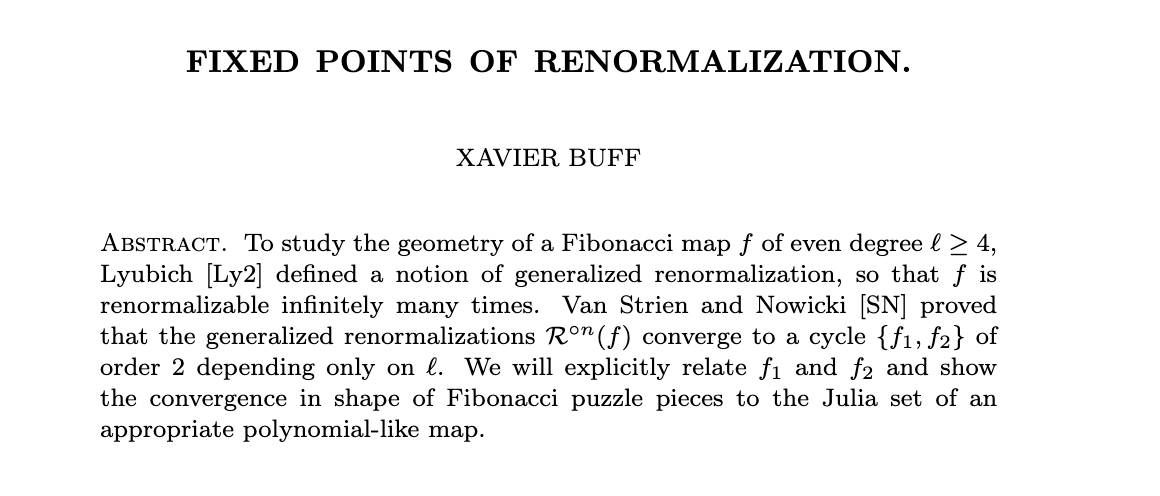
不过,Xavier Buff针对Fibonacci Maps还是撰写了一篇英文的文章《FIXED POINTS OF RENORMALIZATION》。他将经典多项式映射的重正化理论拓展至更广泛的映射类型(称为L-映射),特别针对具有特定临界轨道组合结构的斐波那契映射(非经典重正化对象),构建了一个封闭的自洽重正化算子。证明实对称斐波那契映射的迭代重正化序列会收敛到一个二阶周期循环(即两个映射交替互为重正化结果)。这两个映射在临界点邻域内表现相同,而在另一特定区域内则呈现符号相反的对称关系。通过重正化不动点导出关键函数方程(Cvitanović-Feigenbaum方程),并证明其解具有独特的几何性质:解的解析域是由拟圆边界界定的拟盘。由此构造的多项式类映射,其动力系统的Julia集具有拟共形等价性(如等价于某类多项式的朱利亚集或拟圆)。这篇论文虽然提供了一个不错的想法,但是对指出原始论文的Gap帮助有限。
做科研比较痛苦的事情就是思考问题,而且要克服的事情就是每天起床之后要面对一天的失败,毕竟365天起码有300天没有结果。经过我个人的不懈努力,一页一页磨,总算在博士第三年把论文推进到Chapter10。虽然推进的速度相对其他方向慢了许多,但是我在阅读论文的过程中还是把周边的论文都读了个遍,包括但不限于Fibonacci Interval Map、Fibonacci Circle Map、Renormalization Theory、Martingale Theory 等方向的书籍与论文资料,当时给我的感觉就是除了这篇文章没搞定,其他论文都搞定了。而且这篇原始的论文我差不多也花费了快三年的时间,可能是我个人的天分不太够吧。在2021年左右,我在师弟的一篇报道中看到下面这一段话,引用在这里以激励大家努力工作从而做出杰出成果:
接近一年的时间就为了去搞懂一篇论文,这在有的人看来是很不划算的,沈老师却有不同的观点:“ 做数学要能静心来,年轻人花十年时间不去计较得失钻研数学不是件吃亏的事情”,这句话让我内心深受震撼。确实数学研究一直是困难重重,做出好的结果更加不易,大多数时候的付出往往没有收获,计较一时的得失只会犹豫不前。只有不忘初心,才不会愧对自己的人生。 “十年不亏”也成为了我后来学习生活的指路明灯,我相信那句话: “念念不忘,必有回响”。
最近到了2025年,回想起当时的种种,也觉得颇有一番道理。如果只是为了做一个普通的结果,那就最好不要去做了。还是要以核心的论文和课题为目标,只有树立远大的目标,最终才会有一个好的结果。比如说,在研究动力系统的过程中,如果以发表《Annals of Mathematics》为目标,那么说不定最终能发表一篇《Communications in Mathematical Physics》;如果以发表《Communications in Mathematical Physics》为目标,或许可以发表一篇《Ergodic Theory and Dynamical Systems》;如果以发表《Ergodic Theory and Dynamical Systems》为目标,最终可能只会发表一篇《Discrete and Continuous Dynamical Systems》;而如果以《Discrete and Continuous Dynamical Systems》为目标,那么估计最后只能发表国内期刊了。当时我还在读博士的时候,我们私下认为,要想在动力系统领域做下去,博士期间至少得发一篇《Ergodic Theory and Dynamical Systems》这个档次的论文,毕竟这算是动力系统领域的敲门砖,发表了之后就算是正式进入这个领域了。
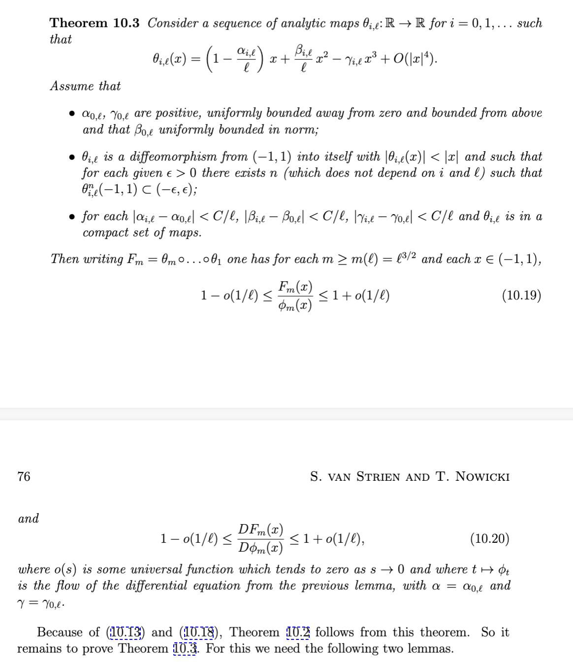
转眼已经是2025年,我再次想起那篇让我头疼了好几年的论文。这一次,我有了一个全新的“助手”——人工智能。我将整篇论文输入到AI中,要求它分析出最有可能出错的关键lemma或theorem。为了避免它被先前的结果干扰,我每次分析前都清空对话历史。第一次,它指向了第10章;第二次,依然是第10章;第三次,依旧如此。这个结果让我震惊,因为十几年前,我也正是凭借自己的直觉和一堆手写演算,将焦点锁定在了那个章节。那一刻,我突然感受到一种跨越时间的验证——仿佛过去那个在热带雨中冥思苦想的我,终于得到了回应。
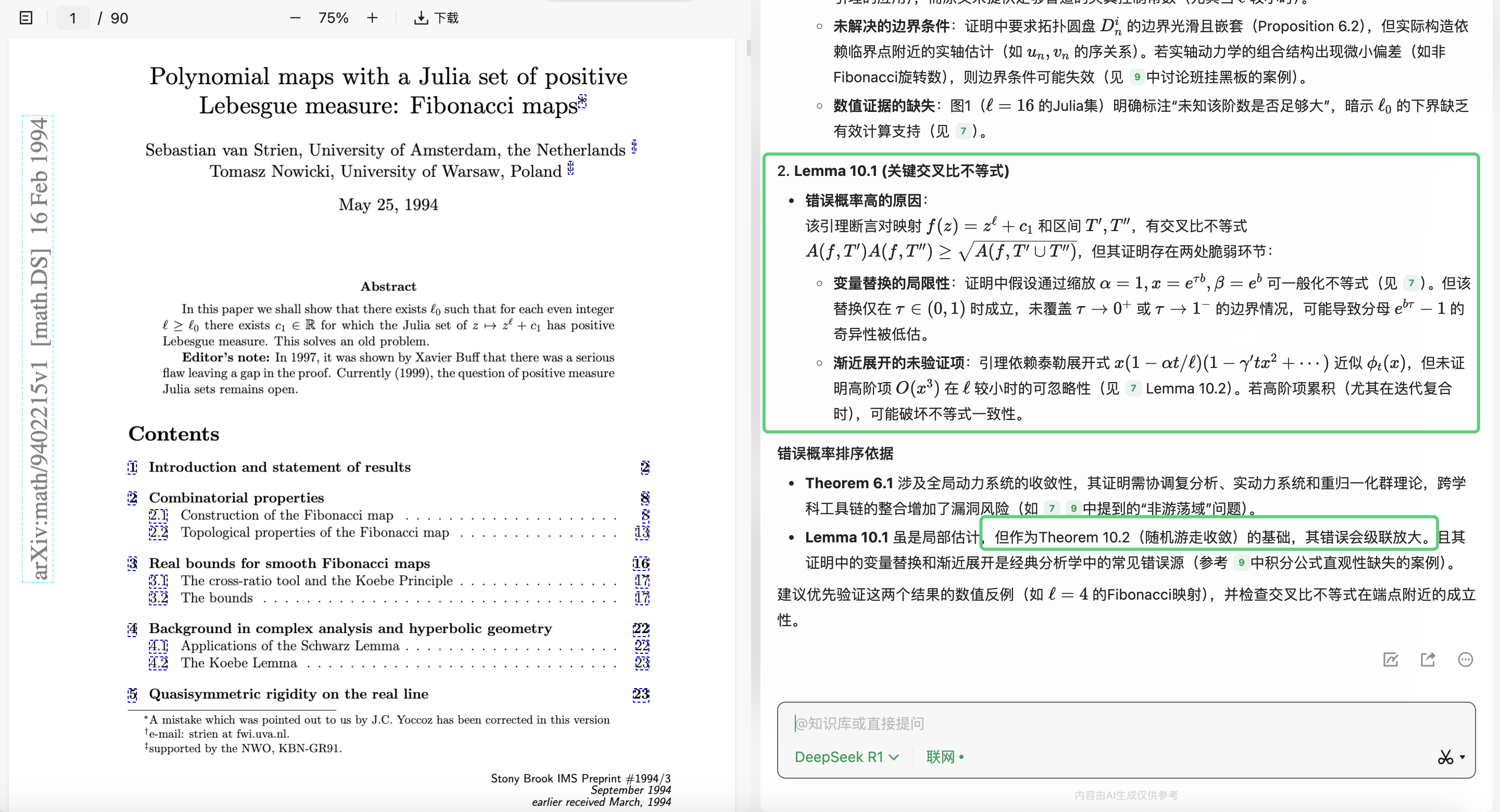
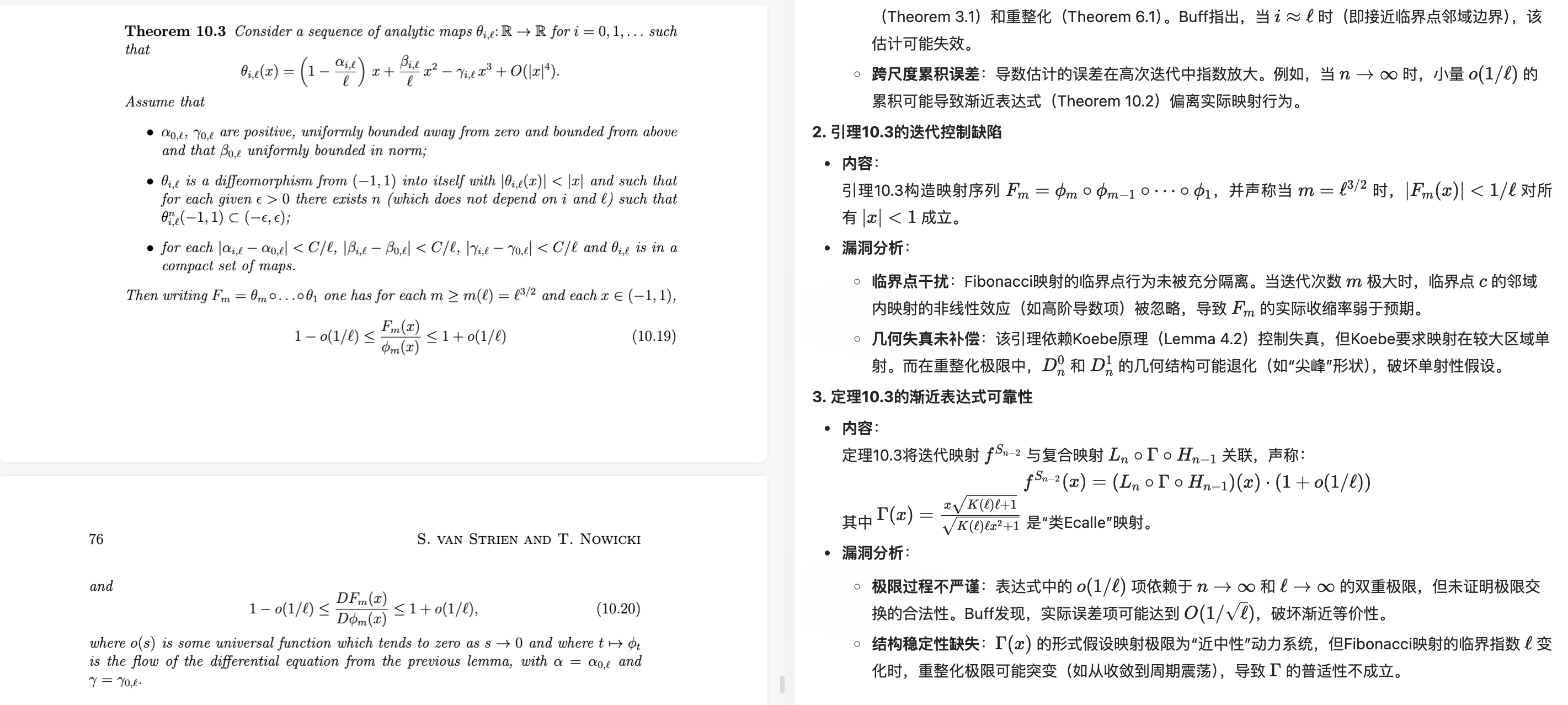
于是,我再次深入提问,追问第10章可能存在的潜在问题。这次,AI指出了引理10.3和定理10.3的渐进表达式可能存在问题,这与我当时认真分析和严格计算得到的初步结果已经非常相似。我意识到,AI并没有直接为我解答问题,它只是以另一种方式验证了我的直觉和判断。那时我可能还在用尺规构建数学的“积木”,而现在,AI则帮我拿起了扫描仪。它不是替代者,而是另一个视角,一个冷静、系统、高效的数学“侦探”。它无法凭空理解抽象背后的意义,但它能以惊人的效率指向结构中的松动之处,让我们这些人类研究者能够更加聚焦地重新思考。
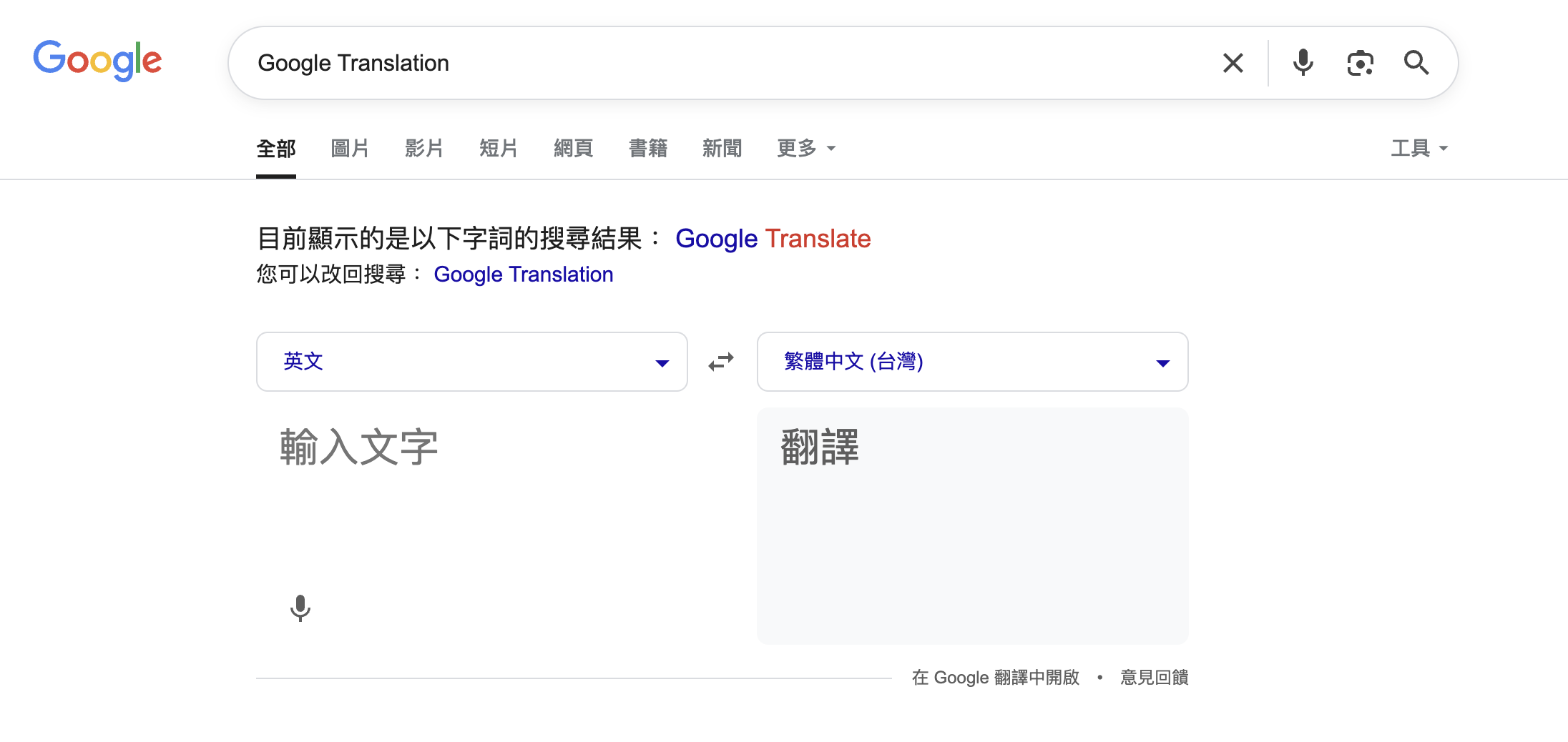
而在2010年我翻译的那一篇法语论文在AI的协助下,翻译变得极为容易,只需要短短几句话,我就可以得到完整的段落翻译,甚至还可以获得论文指出的“Gap”。从论文指出的内容来看,确实也算指出了原始论文存在不可逾越的缺陷。


这次经历让我对之前的科研进行了反思,也对AI的使用有了更深层次的体会。AI可以是导师,是助手,是共谋者,但它永远无法取代我们对于美、逻辑和意义的追求。我记得在新加坡的前三年时间里,我对着这篇论文感到迷茫和无力;而现在,我借助AI,让迷雾稍稍散去了一点。这不仅仅是一次问题的回溯,更像是一次人与技术共舞的实验。最终,我并没有解决那个难题,但我知道,解决的路径已经比过去清晰了许多。
未来的科研,将是人与AI的合奏。我们用直觉和经验提出问题,AI用速度和模式捕捉给出方向。而最终的证明与理解,仍然属于我们。那些新加坡每天准点落下的雷雨,就像是大自然给出的节奏,而AI,是帮我们听懂这段旋律的新耳朵。


 infinite paraboloid
 hyperbolic paraboloid
 sphere with radius
  and center


 cylinder
 Plane
Plane Parabola
 : 1 question. Especially,
  and
and  (Integration by parts).
 : 1 question, where
  is a positive real number. Especially,
  and
and  .
. and reverse the order of dx and dy).
 and the domain
  plane. If the domain
  , where
  . Pay attention to the orientation of the curve on the boundary, i.e. the right hand rule).
 ).
).


 is called a critical point of f(x), if
 on some interval I, then f(x) is increasing on the interval I. Similarly, if
  on some interval I, then f(x) is decreasing on the interval I.
 is
is  where
where  is the slope of the tangent line.
 is
is  because the Chain Rule of derivatives.
 at the point (16,16).
 at the both sides, we get
 That means the tangent line of the curve at the point (16,16) is y-16=-(x-16). i.e. y=-x+32.
 , then calculating the derivative directly. i.e.
 then (16,16) corresponds to
  From the derivative of the parameter functions, we know
 then
then  and
and  Find dy/dx and express your answer in terms of
 ,
,


 is a function with one variable
  with ordinary differential equation
  The solution is
 with some constant
  .
. where
where  is a function with one variable
  and
and  is a function with one variable
 with some constant
 The integrating factor is
  That means
 and take the integration under x at the both sides,
 for some constant
  or
or  , since the following formulas:

 for the first order ordinary differential equation
  then we must make use of the initial condition to calculate the constant C after we solved the equation.
 infinite paraboloid
 cylinder
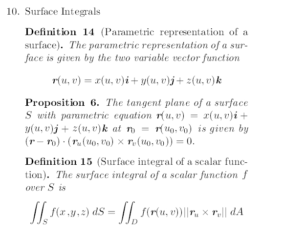
 is a function,
  is a surface S. Then the surface integral is
 denotes the cross product between
  and
and  ,
, denotes the length of the vector
 for all
  , and
, and 
 , since
 and
and  the cross product

 , such that
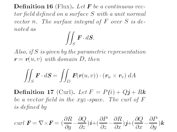
  determines the velocity of the fluid at
  . The flux is defined as the quantity of fluid flowing through
  does not just flow along
  has both a tangential and a normal component, then only the normal component contributes to the flux. Based on this reasoning, to find the flux, we need to take the dot product of
 is a vector field,
 is a scalar function. That means,

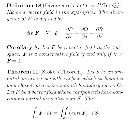
 is a bounded domain and
 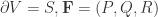 is a vector field.
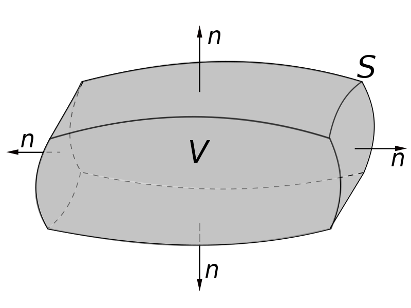

 is a vector field.
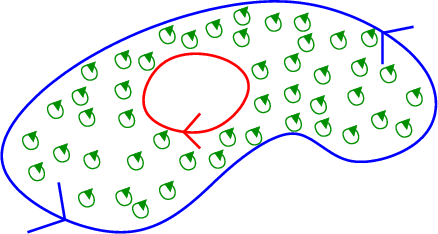
  is a compact surface and
  is the boundary of
  The curve
  has the positive orientation, that means following the right hand rule.
 is a smooth function,
 is the domain of
  .
.
![r:[a,b] \rightarrow C](https://s0.wp.com/latex.php?latex=r%3A%5Ba%2Cb%5D+%5Crightarrow+C+&bg=ffffff&fg=2b2b2b&s=1&c=20201002) is a smooth curve.
is a smooth curve. is a smooth vector function,
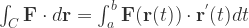
 is a vector field,
 is the domain and
  denotes the boundary of
  The orientation of
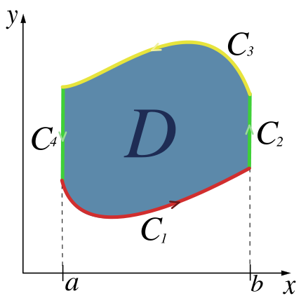
 , the orientation is counterclockwise.
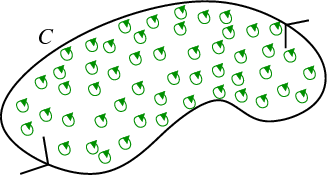
 denotes the area of


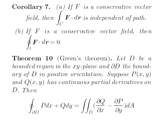
 is called a conservative vector field, if there exists a scalar field
  . It is equivalent to these conditions:

 .
.
 depends only on the initial point and terminal point of the curve
  and
and  have the same initial points and terminal points, then these two line integrals are equal:
  . For this reason, a line integral of a conservative vector field is called path independent.
 , let
, let  denote the curve
  , where
  Let
Let
 in the domain
 ,
,  ,
,  ,
,


 on
on  .
. .
. the
the 
 bounded by
  and
and 
 and
and 


 is
is  the minimum value is taken at
 .
.


 on
on 

 where
where 


 is
is  .
.


 is a conservative vector field. Since


 is a conservative vector field, and we can assume
  , i.e.
  Hence,
 for some constant


 and
and  with
with 
 it is counterclockwise,
 is from 0 to
 it is clockwise,
 to 0.
to 0. ,
,


 , the domain
 and
and  are partial derivatives of
  and
and  respectively.
 and the projection of it on


 the function


 is
is 

 the volume of the ellipsoid is

 and
and  the determinant of Jacobian matrix is

 or 0/0, then we can use the L.Hospital Rule to calculate the limit. Precisely, the L.Hospital Rule is
 is a differentiable function and its derivative
  .
.

 .
.


 .
. .
.


 .
.


 where y=1/x.
 where a>0.
 is
is


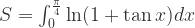
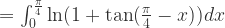
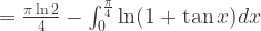
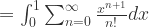
 . Calculate the value of S.


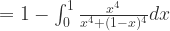
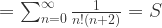
 to show that S=1.
 is
is  . Take the integration of the function on the interval [0,1], we get

 .
. .
. is
is  . Differentiate f(x) and get
  . Moreover,
  and
and  .
. This implies f(0)=0. Assume
 we get
  That means f(1)=1.
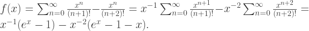 Therefore, f(1)=1.
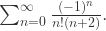 Answer is

 .
.


 .
.


 .
. ,
,


 and
and  .
.