Category Archives: DeepMind

Value iteration networks

Value Iteration Networks Tamar et al., NIPS 2016

‘Value Iteration Networks’ won a best paper award at NIPS 2016. It tackles two of the hot issues in reinforcement learning at the moment: incorporating longer range planning into the learned strategies, and improving transfer learning from one problem to another. It’s two for the price of one, as both of these challenges are addressed by an architecture that learns to plan.

In the grid-world domain shown below, a standard reinforcement learning network, trained on several instances of the world, may still have trouble generalizing to a new unseen domain (right-hand image).

(This setup is very similar to the maze replanning challenge in ‘Strategic attentive writer for learning macro actions‘ from the Google DeepMind team that we looked at earlier this year. Both papers were published at the same time).

… as we show in our experiments, while standard CNN-based networks can be easily trained to solve a set of such maps, they do not generalize well to new tasks outside this set, because they do not understand the goal-directed nature of the behavior. This observation suggests that the computation learned by reactive policies is different from planning, which is required to solve a new task.

Planning is not a new problem – the value iteration algorithm based on Markov decision processes (MDP) has been known since 1957! What Tamar et al. do in this work though, is embed a value iteration (VI) planning component inside the overall neural network architecture. And the breakthrough insight is that the VI algorithm itself can be encoded by a specific type of CNN, which means it is differentiable.

By embedding such a VI network module inside a standard feed-forward classification network, we obtain an NN model that can learn the parameters of a planning computation that yields useful predictions. The VI block is differentiable, and the whole network can be trained using standard backpropagation.

It really is pretty cool – you give the network the machinery that can be used for planning, and it figures out all by itself the best way to use it.

Using the approach, Tamar et al. show that value iteration networks (VINS) generalize better to new grid-world scenarios than either CNNs following the DQN architecture, or fully convolutional networks (FCNs):

(Note there is no comparison to the contemporary STRAW architecture from the DeepMind team that also extends DQNs with planning).

Importantly, note that the prediction loss for the reactive policies is comparable to the VINs, although their success rate is significantly worse. This shows that this is not a standard case of overfitting/underfitting of the reactive policies. Rather, VIN policies, by their VI structure, focus prediction errors on less important parts of the trajectory, while reactive policies do not make this distinction, and learn the easily predictable parts of the trajectory yet fail on the complete task.

They also demonstrated planning success using Mars landscape images for Mars Rover navigation, planning in a physical simulation setting, and planning in the WebNav setting which requires navigating links of a web site towards a goal page.

What I’d love to see is how well the VIN architecture performs on theFrostbite Challenge.

Let’s take a closer look at how it all works, starting with the value iteration algorithm itself, then how to encode that in a NN, before finally putting it all together in a complete architecture.

Standard value iteration

“A standard model for sequential decision making and planning is the Markov Decision Process (MDP).”

You have a set of states s \in S, a set of actions a \in A, a reward function R(s,a) that gives the anticipated reward for taking action a in state s, and atransition kernel, P(s'|s,a) that encodes the probability of the next state given the current state and action. A policy \pi(a|s) prescribes the action distribution for each state.

(Note the similarity between this structure and the action matrix of STRAW).

The goal in an MDP is to find a policy that obtains high rewards in the long term.

You can consider the value of a state under some policy as the expected discounted sum of rewards when starting from that state and following the policy. A optimal policy will find the maximal long-term return possible from a given state. Value iteration computes the rewards by iterating over the action steps (\gamma \in (0,1) is a discount factor):

Encoding value iteration in a neural network

Our starting point is the VI algorithm (1). Our main observation is that each iteration of VI may be seen as passing the previous value function Vn and reward function R through a convolution layer and max-pooling layer. In this analogy, each channel in the convolution layer corresponds to the Q-function for a specific action, and convolution kernel weights correspond to the discounted transition probabilities. Thus by recurrently applying a convolution layer K times, K iterations of VI are effectively performed.

This idea leads to the following network structure:

A reward ‘image’ \bar{R} (to follow the more normal CNN formulation of working with images) is fed into convolutional layer \bar{Q} with \bar{A} channels. Each channel corresponds to \bar{Q}(\bar{s},\bar{a}) for action \bar{a}. The layer is max-pooled along the actions channel to produce the next-iteration value function layer. This is stacked with the reward \bar{R} and fed back in K times, to performK iterations of value iteration.

The full Value Iteration Network model

The value-iteration module we just described can now be embedded into a full value iteration network as follows:

In many systems, if you’re in a given state, and you take a given action, the set of possible states you end up in is much smaller than the overall universe of states. More precisely, the the states for which \bar{P}(\bar{s'}|\bar{s},\bar{a}) > 0 is a small subset of \bar{S}.

In NN terminology, this is a form of attention, in the sense that for a given label prediction (action), only a subset of the input features (value function) is relevant. Attention is known to improve learning performance by reducing the effective number of network parameters during learning.

This is the purpose of the attention module added into the feedback loop in the diagram above. With the inclusion of the CNN-based value iteration module, everything in the value iteration network is differentiable:

This allows us to treat the planning module as just another NN, and by back-propagating through it, we can train the whole policy end-to-end.

To implement a VIN, you need to specify the state and action spaces for the planning module (\bar{S} and \bar{A}), the reward functions f_R and f_P, and the attention function. The authors call this the process of VIN design.

Once a VIN design is chose, implementing the VIN is straightforward, as it is simply a form of CNN. The networks in our experiments all required only several lines of Theano code.

Advertisement

[转载]强化学习系列之九:Deep Q Network (DQN)

我们终于来到了深度强化学习。

reinforcement learning

1. 强化学习和深度学习结合

机器学习=目标+表示+优化。目标层面的工作关心应该学习到什么样的模型,强化学习应该学习到使得激励函数最大的模型。表示方面的工作关心数据表示成什么样有利于学习,深度学习是最近几年兴起的表示方法,在图像和语音的表示方面有很好的效果。深度强化学习则是两者结合在一起,深度学习负责表示马尔科夫决策过程的状态,强化学习负责把控学习方向。

深度强化学习有三条线:分别是基于价值的深度强化学习,基于策略的深度强化学习和基于模型的深度强化学习。这三种不同类型的深度强化学习用深度神经网络替代了强化学习的不同部件。基于价值的深度强化学习本质上是一个 Q Learning 算法,目标是估计最优策略的 Q 值。 不同的地方在于 Q Learning 中价值函数近似用了深度神经网络。比如 DQN 在 Atari 游戏任务中,输入是 Atari 的游戏画面,因此使用适合图像处理的卷积神经网络(Convolutional Neural Network,CNN)。下图就是 DQN 的框架图。

dqn-atari

2. Deep Q Network (DQN) 算法

当然了基于价值的深度强化学习不仅仅是把 Q Learning 中的价值函数用深度神经网络近似,还做了其他改进。

这个算法就是著名的 DQN 算法,由 DeepMind 在 2013 年在 NIPS 提出。DQN 算法的主要做法是 Experience Replay,其将系统探索环境得到的数据储存起来,然后随机采样样本更新深度神经网络的参数。

experience_replay

Experience Replay 的动机是:1)深度神经网络作为有监督学习模型,要求数据满足独立同分布,2)但 Q Learning 算法得到的样本前后是有关系的。为了打破数据之间的关联性,Experience Replay 方法通过存储-采样的方法将这个关联性打破了。

DeepMind 在 2015 年初在 Nature 上发布了文章,引入了 Target Q 的概念,进一步打破数据关联性。Target Q 的概念是用旧的深度神经网络 w 去得到目标值,下面是带有 Target Q 的 Q Learning 的优化目标。

J=min(r+γmaxaQ(s,a,w))Q(s,a,w))2

下图是 Nature 论文上的结果。可以看到,打破数据关联性确实很大程度地提高了效果。

nature-result

3. 后续发展

DQN 是第一个成功地将深度学习和强化学习结合起来的模型,启发了后续一系列的工作。这些后续工作中比较有名的有 Double DQN, Prioritized Replay 和 Dueling Network。

3.1 Double DQN

Thrun 和 Schwartz 在古老的 1993 年观察到 Q-Learning 的过优化 (overoptimism) 现象 [1],并且指出过优化现象是由于 Q-Learning 算法中的 max 操作造成的。令 Qtarget(s,a) 是目标 Q 值;我们用了价值函数近似,Qapprox 是近似 Q 值;令 Y 为近似值和目标之间的误差,即

Qapprox(s,a)=Qtarget(s,a)+Ys,a

Q-learning 算法更新步骤将所有的 Q 值更新一遍,这个时候近似值和目标值之间的差值

Z==rs,a+γmaxa1Qapprox(s,a1)rs,a+γmaxa2Qtarget(s,a2)γmaxa1Qapprox(s,a1)γmaxa2Qtarget(s,a2)γQapprox(s,a)Qtarget(s,a)=γYs,a(1)

其中 a=argmaxaQtarget(s,a)。这时候我们发现,即使 E[Y]=0 也就是一开始是无偏的近似, Q Learning 中的 max 操作也会导致 E[Z] > 0。这就是过优化现象。为了解决这个问题,Thrun 和 Schwartz 提出了 Double Q 的想法。      Hasselt 等进一步分析了过优化的现象,并将 Double Q 的想法应用在 DQN 上,从而提出了 Double DQN。Double DQN 训练两个 Q 网络,一个负责选择动作,另一个负责计算。两个 Q 网络交替进行更新,具体算法如下所示。

double-q-algorithm

下图是 Hasselt 在论文中报告的实验结果。从实验结果来看,Double DQN 拥有比 DQN 好的效果。

double_dqn

3.2 Prioritized Replay

DQN 用了 Experience Replay 算法,将系统探索环境获得的样本保存起来,然后从中采样出样本以更新模型参数。对于采样,一个常见的改进是改变采样的概率。Prioritized Replay [3] 便是采取了这个策略,采用 TD-err 作为评判标准进行采样。

TDerr=|rs,a+γmaxaQ(s,a)Q(s,a)|(2)

下图是论文中采用的例子。例子中有 n 个状态,在每个状态系统一半概率采取 “正确” 或者一半概率 “错误”,图中红色虚线是错误动作。一旦系统采取错误动作,游戏结束。只有第 n 个状态 “正确” 朝向第 1 个状态,系统获得奖励 1。在这个例子训练过程中,系统产生无效样本,导致训练效率底下。如果采用 TD-err 作为评判标准进行采样,能够缓解这个问题。

priorized-example

论文报告了 Prioritized Replay 算法效果。从下图来看,Prioritized Replay 效果很好。

prioritized

3.3 Dueling Network

Baird 在 1993 年提出将 Q 值分解为价值 (Value) 和优势 (Advantage) [4]。

Q(s,a)=V(s)+A(s,a)

这个想法可以用下面的例子说明 [5]。上面两张图表示,前方无车时,选择什么动作并不会太影响行车状态。这个时候系统关注状态的价值,而对影响动作优势不是很关心。下面两张图表示,前方有车时,选择动作至关重要。这个时候系统需要关心优势了。这个例子说明,Q 值分解为价值和优势更能刻画强化学习的过程。

value-advantage

Wang Z 将这个 idea 应用在深度强化学习中,提出了下面的网络结构 [5]。

dueling-structure

这种网络结构很简单,但获得了很好的效果。

dueling

Dueling Network 是一个深度学习的网络结构。它可以结合之前介绍的 Experience Replay、 Double DQN 和 Prioritized Replay 等方法。 作者在论文中报告 Dueling Network 和 Prioritized Replay 结合的效果最好。

4. 总结

上次本来想把基于价值的深度强化学习的 Double DQN, Prioritized Replay 和 Dueling Network 也写了的,写到晚上 2 点。现在补上这部分内容。

从上面介绍来看,DQN、 Double DQN、Prioritized Replay 和 Dueling Network 都能在深度学习出现之前的工作找到一些渊源。深度学习的出现,将这些方法的效果提高了前所未有的高度。

文章结尾欢迎关注我的公众号 AlgorithmDog,每次更新就会有提醒哦~

weixin_saomiao


[1] S. Thrun and A. Schwartz. Issues in using function approximation for reinforcement learning. In M. Mozer, P. Smolensky, D. Touretzky, J. Elman, and A. Weigend, editors, Proceedings of the 1993 Connectionist Models Summer School, Hillsdale, NJ, 1993. Lawrence Erlbaum.
[2] Van Hasselt, Hado, Arthur Guez, and David Silver. “Deep reinforcement learning with double Q-learning.” CoRR, abs/1509.06461 (2015).
[3] Schaul T, Quan J, Antonoglou I, et al. Prioritized experience replay[J]. arXiv preprint arXiv:1511.05952, 2015.
[4] Baird, L.C. Advantage updating. Technical Report WLTR-93-1146,
Wright-Patterson Air Force Base, 1993.
[5] Wang Z, de Freitas N, Lanctot M. Dueling network architectures for deep reinforcement learning[J]. arXiv preprint arXiv:1511.06581, 2015.

强化学习系列系列文章

此条目发表在强化学习分类目录,贴了标签。将固定链接加入收藏夹。

2016年的AI,一场史无前例的技术营销

版权归作者所有,任何形式转载请联系作者。
作者:insightlight(来自豆瓣)
来源:https://www.douban.com/note/602333108/

2016年12月29日,大概又是一个会被载入史册的日子。名叫SkyNet,哦不,是”Master”的围棋AI,开始了第一次对人类的血洗。

在奕城的第一晚,Master十战全胜;第二日,横扫韩国第一人朴廷桓九九段、世界第一人柯洁,比分都是2比0;第三日,陈耀烨九段、金庭贤五段、范廷钰九段、芈昱廷九段和唐韦星九段依次落马;再之后是古力、时越、金志锡、井山裕太;到了1月4日,聂卫平老先生以7目半落败。最终战绩,Master 60胜0负1平(平的那局是因为掉线)

自此,Artificial Intelligence(AI),这个在2016年已经如日中天的buzzword,再一次传遍大街小巷。人们沉浸在对AI的崇拜、慌乱与恐惧之中,然而作为吃瓜群众的笔者却在想一个问题:如果DeepMind没有事先与各国棋院通气,整个事件如何能进行得如此顺利,在时间上如此紧凑?所有重要的世界高手,都在短短几天的时间窗口内腾出了时间,如果说没有提前策划和组织,实在有点难以置信。掐指一算自从3月份AlphaGo的横空出世,DeepMind已有9个月时间没有在圈外露脸,大概它也感受到了营销的压力吧。

其实纵观2016年,在阿尔法狗狗的带领之下,AI界隔三差五地在圈内外制造着骚动:3月,除了人尽皆知的AlphaGo事件,李开复关于人工智能博士200w+美金年薪的文章刷屏;4月,Google著名的深度学习框架TensorFlow发布分布式版本;6月,Prisma上线,红极一时;8月,Google发布基于深度学习的NLU框架SyntaxNet; 9月,Google上线基于深度学习的机器翻译,索尼用人工智能写了两首歌;11月,计算机视觉学术大牛李飞飞老师下海进入工业界;12月,百度宣布他们的深度学习系统在语音识别上超过人类,DeepMind在NIPS16会议上宣布DeepMind Lab开源。一切的一切,都在各大媒体冠以【重磅】开头的新闻标题之下,一次次地牵动着广大吃瓜群众的神经——然而这些成就实际上离我们的生活又是那么的遥远。

在科技的历史上,从未有任何一项科技,在它的大规模真实应用之前,有持续一年甚至几年的营销运动。在这个风口之上,在这个AI几年的造势运动把人们的期望与恐惧推上一个历史顶点,而其真正落地应用又遥遥无期的一个尴尬节点,是时候冷静下来回顾一下AI的营销史了。

一、一些概念和历史

有几个概念需要先明确一下,因为我发现在今日媒体的狂轰滥炸之下,有大批AI民科是分不清像“人工智能”、“机器学习”、“深度学习”这些概念的关系的(例如我认识的非科班出身的人有90%认为机器学习=深度学习)。当然这些概念的含义也一直在“与时俱进”,不过学界还是有一个相对统一且合理的认知,可以帮助我们阐述问题。下面这张图描述了其中最重要的几个概念之间的关系
“人工智能”这个buzzword,常常会因为营销或者新闻报道的需求而被赋予不同的含义,其外延有时等同于“机器学习”,有时不等同,所以最外圈的这个等号并不完全准确。不过在2016年被大家普遍讨论的这些“AI”,可以认为基本上就是机器学习。内部的四个小圈则是学术上有确定外延的四个概念,代表了当前最重要的四个问题领域,是需要明确的重点概念。

有监督学习(supervised learning)——让机器观测到一些输入,并告诉机器在这些输入下应该产生什么样的输出。机器通过这些数据学习出一个模型,之后给它新输入的时候,它能够根据模型预测应该产生什么样的输出。比如机器看到一个图片,可以判断图片中的物体属于哪一个分类。

无监督学习(unsupervised learning)——让机器观测到一些输入,而没有标准输出,让机器自行去总结这些输入数据有什么统计特征,并生成有意义的产出。例如自动把大批文章聚成相似的几类,又例如给计算机看一些小狗小猫的照片,让计算机自动生成一些新的(与看过的相似但又不同的)小狗小猫的照片。

增强学习(reinforcement learning)——让机器观测到一些输入,并让机器根据输入做特定动作(action)。这些动作导致机器获得收益或者惩罚(reward)。机器通过增强学习优化它的动作策略(strategy),使得它的长期收益最大化。下棋就是这一类典型的问题,strategy就是行棋策略,reward就是赢棋。

深度学习(deep learning)——事实上不是一类问题,而只是一种方法,一种通过多层神经网络来构建上述三种问题所需要的模型的方法。

回到历史。这一波的AI热,最早应归功于Hinton老头子的文章《A fast learning algorithm for deep belief nets》这篇文章是2005年写的,截至2017年1月14日已有5000+的引用,足见其影响力)这篇文章实际上是用一种无监督学习的方法实现了对原始数据逐层抽取深度特征,而这些深度特征可以被用为有监督学习的特征来提高有监督学习的准确率。这解决了长久以来神经网络“无法做深”的痛点(原因是训练信号会随着深度增加而被稀释,有兴趣的读者可查阅相关资料),算是一个比较大的贡献。不过当时这个文章传达的大方向是用无监督学习的方法抽取特征(这个过程叫做pre-training),并没有把重点放在有监督学习本身的模型上,所以当时的同学们对于有监督/无监督在方向选择上是有点迷茫的。

这种迷茫直到2012年还存在。这一年的一件大事是Andrew NG等人的Google Brain团队,搞了一个庞大的分布式深度学习,在ImageNet图片物体分类竞赛中把对手远远甩在了身后(《Building High-level Features Using Large Scale Unsupervised Learning》)前面已经说过,物体分类是一个有监督学习任务,但是由于Hinton老爷子定下的无监督学习基调,Andrew NG等人还是把重心放在了无监督学习生成特征上面,并且做出了那幅著名的“机器学习出来的猫”。有趣的是,在2012年的NIPS上,Hinton和NG的团队同时放弃了pre-training。失去了pre-training的帮助,就需要其他方法解决训练信号被稀释的问题,Hinton团队的方法是换了一种叫做ReLU的激活函数( 《ImageNet Classification with Deep Convolutional Neural Networks 》),NG团队的方法则是怼机器,大量的机器(《Large Scale Distributed Deep Networks》)。Hinton团队同时还抛出了CNN应用到ImageNet上的表现,CNN和ReLU这两个东西非常重要,成为此后深度学习研究的标配。结果Hinton团队这篇文章的引用数有8000多,而NG团队的两篇分别是700多和1000多。NG的营销能力强,学术创新上却总是比Hinton老爷子慢半拍。Anyway,自从12年NIPS这两篇文章之后的一段时间,大家对无监督学习就不怎么感冒了。
2012年Andrew NG团队无监督学习生成的猫脸图片。图片来源:New York Times
也是从2012年的ImageNet竞赛开始,AI进入第一个营销高潮。当时的人们对于计算机识别小猫小狗这种事情还觉得很新鲜,于是接下来科研圈的开始对此类事情趋之若鹜。几乎每个做机器学习的实验室都会尝试一把在State-of-the-art的模型上做一点哪怕是很小的微创新,希望能产生ImageNet准确率上一点哪怕是很小的提升,一旦成功了,就可以说自己是新的State-of-the-art。从那以后,大家开始只关心实验的准确率,越来越少的人关心模型本身的理论价值。AI研究的方法论,从传统科学的重视推理论证,变成了快速尝试+总结相关性(也就是所谓的“大数据思维”)。毕竟准确率数字是很好拿出去说的,理论价值却很难讲清楚。 AI自此进入营销时代。

在AI学术界这一翻天覆地的变化背后,Andrew NG功不可没。深度学习理论上的重要突破大多都不是归属于他的,然而他做了几件重要的事情:2008年发起“Stanford Engineering Everywhere”(SEE)项目,把自己的机器学习课程曝光给全世界人民;2011年组建了Google Brain项目,这个项目初期的最主要产出之一就是后来被媒体大书特书的那张无监督学习出来的猫脸,并且这个结果在报道的时候给人一种“机器有了自主学习能力”的认知;2012年创立Coursera,在MOOC社区中进一步营造出一种AI大繁荣的景象。NG大概是这几年媒体出镜率最高的AI学术圈人士。与其说是一位科学家,Andrew NG的角色更像是一位优秀的AI产品经理及营销人员,他的营销能力在圈内早已得到公认。关于NG的营销能力,在NIPS 2016会议上还有一个有趣的小细节,将会在后面提到。

回到我们的时间线,鉴于2012年底深度学习在有监督学习上的巨大成功,一段时间内大家忙于把这项技术推广到各个应用领域跑马圈地(其实主要还是图像和语音),暂时忘掉了无监督学习和生成猫脸的事情。到了2014年,当各个领域都被圈的差不多了,学术界在苦苦寻找下一个噱头的时候,大神Ian Goodfellow通过一个叫做“干”的东西(GAN,Generative Adversarial Network)把无监督学习重新带回了人们的视线。“干”干的就是“给计算机看一些小狗小猫的照片,让计算机自动生成一些新的(与看过的相似但又不同的)小狗小猫的照片”这样一件事情,不同点在于,它干的非常不错。一时间,AI学术界迅速高潮了,纷纷竞争起生成图片(以及语音、音乐等各种其他东西)的生意来。大家也并不关心我们为什么需要生成这些图片(相比之下语音合成和自动生成音乐反而更容易理解一些),大概只是觉得“能干这件事情看起来就很牛逼”,于是就做了,而且做的越来越好。下图是Ian Goodfellow在NIPS 2016上讲GAN的Tutorial里展示的一个生成小动物的demo(《NIPS 2016 Tutorial: Generative Adversarial Networks》)。
GAN生成的小动物图片。图片来源:Ian Goodfellow, NIPS 2016 Tutorial: Generative Adversarial Networks
与此同时,DeepMind在增强学习上的努力,则一直在相对低调地进行。增强学习在很长一段时间内被认为是“仅停留在学术研究”的存在,因其难以降下来的巨大状态空间和动作空间,很难做出一个可展示又足够吸引吃瓜群众的demo。因而在AlphaGo诞生之前,增强学习的研究一直处于一个不温不火的状态。一个叫做“DQN”的东西的出现打破了这个局面。通过把深度学习应用在strategy的学习更新上,巧妙避开大状态空间和动作空间,DQN使得在一个相对小的多的参数空间内训练成为可能(《Playing Atari with Deep Reinforcement Learning》)。这是一个了不起的成就,为后来的AlphaGo奠定了基础。这个伟大想法产生的时间在2013年以前(前述文章在2013年发表),而直到2015年AlphaGo问世之后才被广为传颂。可见一个漂亮的demo是多么重要。

再然后,就是大家都知道的事情了。

二、一些奇怪的现象

AI围棋战胜人类,本身是一个伟大的成就。然而在这个伟大浪潮推动下的AI学术大跃进与创业热中,却出现了很多奇怪的现象。

理性地分析AI这个事情,至少应该提三个问题:1. 这玩意到底做不做的出来;2. 假如这玩意能做出来,那么它做出来以后到底有没有应用前景;3. 假如这玩意能做出来且有应用前景,它会不会毁灭人类。这三个问题是层层递进的关系,对1的答案是肯定的讨论2才有意义,对2的答案是肯定的讨论3才有意义。于是有了第一个奇怪的现象:大部分的吃瓜群众,直接跳过了1、2而去关注3。甚至他们中的乐观主义者,直接跳过123,开始充满自信地迎接这个“未来趋势”了。是Alpha狗狗给我们的信心过于足了吗?

要知道,真正的AI工作者甚至对问题1都没有足够的自信。不错,AlphaGo毫无疑问“已经做出来了”,但不要忘了,围棋再复杂,它仍然是一个游戏;从一个两页纸即可将规则全部讲明的游戏到一个充斥着复杂场景的现实世界,有着巨大的鸿沟需要跨越。在NIPS 2016上,可以明确地感受到,DeepMind已经处在一个深陷游戏之中无法自拔的尴尬状态——不仅几乎所有的paper都是以游戏为demo的,甚至有些研究的目标都是奔着游戏而去的(例如有的工作研究人类玩游戏时是否用到了先验知识,有的工作研究人类玩游戏时的学习曲线,分的很细)。游戏在这些的研究中并不只是一个用来展示的demo,而就是研究的核心。DeepMind在AlphaGo之后一直宣称的进军医疗这件事,却在NIPS 2016上几乎不被人提起。

有意思的是,擅长营销的Andrew NG在NIPS 2016的演讲还趁机轻踩了一下他不太涉足的无监督学习和增强学习。他在白板上画了这样三条曲线。
意思是说,有监督学习的应用在2011年起步,到现在已经比较成熟了;无监督学习刚刚起步;增强学习的真实应用则还是遥远的未来。虽然脱不开为自己营销之嫌,这个说法本身还是比较靠谱的。连李开复也在几天前发的一篇长文《AI创业的十个真想》中,白纸黑字地说到“AlphaGo本身没有商业价值”。像下围棋这样的增强学习技术应用到真实的生活生产,产生游戏之外的价值,不说是一个遥远的未来,至少还是一个技术上比较不确定的事情。

第二个奇怪是没有人问问题2。普通人并不奇怪,奇怪的是产品经理这样一群人,他们在平日工作中对一个产品的应用前景的拷问,可以苛责到极致;而到了AI这件事上,却看不到一篇在产品技术层面客观剖析应用前景的文章。一个最明显的例子是最近大热的聊天机器人。不知道“聊天机器人将是下一代的操作系统”这样一个牛皮是如何在业界传播开来的?再重复一遍,“聊天机器人将是下一代的操作系统”,这话听上去就需要很多解释和论证吧?反正每当我在一个网站正常服务点不进去,不得不求助在线客服或者是电话客服(指人工客服)的时候,就已经很不爽了。当然不是说别人想法都和我一样,但是对于一个与用户直接交互的界面,是不是至少应该做个用户调研,再说“聊天机器人将是下一代的操作系统”这样的话?

第三个奇怪有关成本。Facebook围棋项目负责人田渊栋前日在自乎专栏上写过这样一段文字:

“在八月份美国围棋大会上,我有幸见到了AlphaGo的主要贡献者黄士杰(AjaHuang)和樊麾。我问他们,我们用了大概80到90块GPU来训练模型,我是否可以在演讲时说我们用了AlphaGo百分之一的GPU?那时Aja神秘地笑了笑说:具体数字不能讲。不过,也许小于百分之一吧。”

一块GPU大约两万人民币,算算总共要花多少钱吧。这还远不是全部,还有以月记的计算时间、电力/带宽消耗,以及那么多份200w美金的工资。

当然这样估算成本未必科学。我想表达的是,唯独在AI这件事上,人们似乎表达出了对于成本问题前所未有的宽容。这宽容体现在除了真正在一线做AI的工程师,极少有人关注成本问题。另外需要澄清的是这里疑问的点是“人们不关注”,并不是想表达“AlphaGo劳民伤财了”这个意思。个人内心里其实是把AlphaGo当做一件伟大的艺术品来看待的,而艺术品是无价的——只有在讨论艺术品的时候可以用“无价”这个度量,对于商业产品不行。

三、该怎么看待这件事情

不要预期过高,不要预期过高,不要预期过高。泡沫时代的我们已经习惯了对未来事物预期过高。被透支的预期甚至成了维持经济的重要支柱。只是每一次泡沫破灭都会很疼。很怀念曾经那个时代,在那个时代里,科学技术的进步源于对真理的信仰与热爱,而不是为了填补预期与现实的反差。然而那个时代已经回不去了。

勤奋一些,学习真相。巴菲特从来不投资自己不熟悉的业务。如果不能判断一件事情,那么就应该真正学习它,知道它是什么东西,在积累了足够知识之后做出判断。如果少一些分不清“深度学习”和“机器学习”的关系的人,或许这个世界也会少一些错误的风向。接受无知而被营销者和媒体的观点摆布,是一件非常可怕的事情。就像我们有时不能从政府那里得到真相,在AI这个学界和工业界各种势力利益关系已经非常庞大复杂的领域内,仅凭我们听到的,恐怕很难得到真相。

如果AlphaGo仅仅是AlphaGo,那该多好啊。

【转载】【David Silver强化学习公开课之一】强化学习入门

【David Silver强化学习公开课之一】强化学习入门

【转载请注明出处】chenrudan.github.io

David Silver:http://www0.cs.ucl.ac.uk/staff/d.silver/web/Home.html

本文链接:https://chenrudan.github.io/blog/2016/06/06/reinforcementlearninglesssion1.html

本文是David Silver强化学习公开课第一课的总结笔记。第一课主要解释了强化学习在多领域的体现,主要解决什么问题,与监督学习算法的区别,完整的算法流程由哪几部分组成,其中的agent又包含什么内容,以及解释了强化学习涉及到的一些概念。

本课视频地址:RL Course by David Silver – Lecture 1: Introduction to Reinforcement Learning

本课ppt地址:http://www0.cs.ucl.ac.uk/staff/d.silver/web/Teaching_files/intro_RL.pdf

文章的内容是课程的一个总结和讨论,会按照自己的理解来组织。个人知识不足再加上英语听力不是那么好可能会有一些理解不准的地方,欢迎一起讨论。

建了一个强化学习讨论qq群,有兴趣的可以加一下群号595176373或者扫描下面的二维码。

1

1. 强化学习是什么

强化学习是多学科多领域交叉的一个产物,它的本质就是解决“decision making”问题,即学会自动进行决策。在computer science领域体现为机器学习算法。在Engineering领域体现在决定the sequence of actions来得到最好的结果。在Neuroscience领域体现在理解人类大脑如何做出决策,主要的研究是reward system。在Psychology领域,研究动物如何做出决策,动物的行为是由什么导致的。在Economics领域体现在博弈论的研究。这所有的问题最终都归结为一个问题,人为什么能够并且如何做出最优决策。

强化学习是一个Sequential Decision Making问题,它需要连续选择一些行为,从而这些行为完成后得到最大的收益最好的结果。它在没有任何label告诉算法应该怎么做的情况下,通过先尝试做出一些行为得到一个结果,通过判断这个结果是对还是错来对之前的行为进行反馈,然后由这个反馈来调整之前的行为,通过不断的调整,算法能够学习到在什么样的情况下选择什么样的行为可以得到最好的结果。

强化学习与监督学习有着不少区别,首先监督学习是有一个label的,这个label告诉算法什么样的输入对应着什么样的输出,而强化学习没有label告诉它在某种情况下应该做出什么样的行为,只有一个做出一系列行为后最终反馈回来的reward signal,这个signal能判断当前选择的行为是好是坏。其次强化学习的结果反馈有延时,有时候可能需要走了很多步以后才知道以前的某一步的选择是好还是坏,而监督学习做了比较坏的选择会立刻反馈给算法。强化学习面对的输入总是在变化,输入不像监督学习是独立同分布的。而每当算法做出一个行为,它影响了下一次决策的输入。

2. 强化学习组成

1

图1 强化学习组成部分(图片来源[1])

强化学习决策流程见上图。需要构造出一个agent(图中的大脑部分),agent能够执行某个action,例如决定机器人超哪个方向走,围棋棋子下在哪个位置。agent能够接收当前环境的一个observation,例如当前机器人的摄像头拍摄到场景。agent还能接收当它执行某个action后的reward,即在第t步agent的工作流程是执行一个动作AtAt,获得该动作之后的环境观测状况OtOt,以及获得这个动作的反馈奖赏RtRt。而环境environment则是agent交互的对象,它是一个行为不可控制的对象,agent一开始不知道环境会对不同action做出什么样的反应,而环境会通过observation告诉agent当前的环境状态,同时环境能够根据可能的最终结果反馈给agent一个reward,例如围棋棋面就是一个environment,它可以根据当前的棋面状况估计一下黑白双方输赢的比例。因而在第t步,environment的工作流程是接收一个AtAt,对这个动作做出反应之后传递环境状况和评估的reward给agent。reward奖赏RtRt,是一个反馈标量值,它表明了在第t步agent做出的决策有多好或者有多不好,整个强化学习优化的目标就是最大化累积reward。例如在射击游戏中,击中敌方的一架飞机,最后的得分会增加,那么这一步的reward就是正值。

3. 一些变量

history是所有动作、状态、奖赏的序列,Ht=A1,O1,R1,,At,Ot,RtHt=A1,O1,R1,…,At,Ot,Rt

environment state,SetSte,环境当前的状态,它反应了环境发生什么改变。这里需要明白的一点是环境自身的状态和环境反馈给agent的状态并不一定是相同的,例如机器人在走路时,当前的environment状态是一个确定的位置,但是它的camera只能拍到周围的景象,无法告诉agent具体的位置,而拍摄到的照片可以认为是对环境的一个observation,也就是说agent并不是总能知道环境是如何发生改变的,只能看到改变后的一个结果展示。

agent state,SatSta,是agent的现在所处状态的表示,它可以是history的任何函数。

information(Markov) state,它包含了history的所有有用信息。一个状态StSt有马尔可夫性质是指下一个时刻的状态仅由当前状态决定,与过去状态无关。这里定义可以看出environment state是有马尔可夫性质的(这个概念不明白可以暂时不管)。

如果说environment是Fully Observable的,那么就是说agent能够直接看到环境当前的状态,在这种情况下agent state与environment state是相等的。而如果说environment是Partially Observable Environments,那么就是上面机器人的那个例子,agent能获取到的不是直接的环境状态。

4. Agent的组成

一个agent由三部分组成Policy、Value function、Model,但这三部分不是必须同时存在的。

Policy,它根据当前看到的observation来决定action,是从state到action的映射。有两种表达形式,一种是Deterministic policy即a=π(s)a=π(s),在某种状态s下,一定会执行某个动作a。一种是Stochastic policy即π(a|s)=p[At=a|St=s]π(a|s)=p[At=a|St=s],它是在某种状态下执行某个动作的概率。

Value function,它预测了当前状态下未来可能获得的reward的期望。Vπ(s)=Eπ[Rt+1+rRt+2+|St=s]Vπ(s)=Eπ[Rt+1+rRt+2+…|St=s]。用于衡量当前状态的好坏。

Model,预测environment下一步会做出什么样的改变,从而预测agent接收到的状态或者reward是什么。因而有两种类型的model,一种是预测下一个state的transition model即Pass=p[St+1=s|St=s,At=a]Pss′a=p[St+1=s′|St=s,At=a],一种是预测下一次reward的reward model即Ras=E[Rt+1|St=s,At=a]Rsa=E[Rt+1|St=s,At=a]

因而根据是否选取这三个部分agent可分为下图中红色字体标出来的五种类型(这里有一个迷宫的例子很好,建议看原视频1:08:10起)。Model Free是指不需要去猜测environment的工作方式,而Model based则是需要学习environment的工作方式。

1

图2 Agent的分类(图片来源[1])

5. 探索和利用

强化学习是一种试错(trial-and-error)的学习方式,一开始不清楚environment的工作方式,不清楚执行什么样的行为是对的,什么样是错的。因而agent需要从不断尝试的经验中发现一个好的policy,从而在这个过程中获取更多的reward。

在这样的学习过程中,就会有一个在Exploration和Exploitation之间的权衡,前者是说会放弃一些已知的reward信息,而去尝试一些新的选择,即在某种状态下,算法也许已经学习到选择什么action让reward比较大,但是并不能每次都做出同样的选择,也许另外一个没有尝试过的选择会让reward更大,即Exploration希望能够探索更多关于environment的信息。而后者是指根据已知的信息最大化reward。例如,在选择一个餐馆时,Exploitation会选择你最喜欢的餐馆,而Exploration会尝试选择一个新的餐馆。

以上是第一课的一些相关内容,主要是介绍了一些基础概念,从而对强化学习有一个基础的认识。

6. 引用

  1. http://www0.cs.ucl.ac.uk/staff/d.silver/web/Teaching_files/intro_RL.pdf

解析 DeepMind 深度强化学习 (Deep Reinforcement Learning) 技术

文/Not_GOD(简书作者)
原文链接:http://www.jianshu.com/p/d347bb2ca53c
著作权归作者所有,转载请联系作者获得授权,并标注“简书作者”。

Two years ago, a small company in London called DeepMind uploaded their pioneering paper “Playing Atari with Deep Reinforcement Learning” to Arxiv. In this paper they demonstrated how a computer learned to play Atari 2600 video games by observing just the screen pixels and receiving a reward when the game score increased. The result was remarkable, because the games and the goals in every game were very different and designed to be challenging for humans. The same model architecture, without any change, was used to learn seven different games, and in three of them the algorithm performed even better than a human!

It has been hailed since then as the first step towards general artificial intelligence – an AI that can survive in a variety of environments, instead of being confined to strict realms such as playing chess. No wonder DeepMind was immediately bought by Google and has been on the forefront of deep learning research ever since. In February 2015 their paper “Human-level control through deep reinforcement learning” was featured on the cover of Nature, one of the most prestigious journals in science. In this paper they applied the same model to 49 different games and achieved superhuman performance in half of them.

Still, while deep models for supervised and unsupervised learning have seen widespread adoption in the community, deep reinforcement learning has remained a bit of a mystery. In this blog post I will be trying to demystify this technique and understand the rationale behind it. The intended audience is someone who already has background in machine learning and possibly in neural networks, but hasn’t had time to delve into reinforcement learning yet.

我们按照下面的几个问题来看看到底深度强化学习技术长成什么样?

  1. 什么是强化学习的主要挑战?针对这个问题,我们会讨论 credit assignment 问题和 exploration-exploitation 困境。
  2. 如何使用数学来形式化强化学习?我们会定义 Markov Decision Process 并用它来对强化学习进行分析推理。
  3. 我们如何指定长期的策略?这里,定义了 discounted future reward,这也给出了在下面部分的算法的基础。
  4. 如何估计或者近似未来收益?给出了简单的基于表的 Q-learning 算法的定义和分析。
  5. 如果状态空间非常巨大该怎么办?这里的 Q-table 就可以使用(深度)神经网络来替代。
  6. 怎么样将这个模型真正可行?采用 Experience replay 技术来稳定神经网络的学习。
  7. 这已经足够了么?最后会研究一些对 exploration-exploitation 问题的简单解决方案。

强化学习

Consider the game Breakout. In this game you control a paddle at the bottom of the screen and have to bounce the ball back to clear all the bricks in the upper half of the screen. Each time you hit a brick, it disappears and your score increases – you get a reward.

图 1:Atari Breakout 游戏:来自 DeepMind

Suppose you want to teach a neural network to play this game. Input to your network would be screen images, and output would be three actions: left, right or fire (to launch the ball). It would make sense to treat it as a classification problem – for each game screen you have to decide, whether you should move left, right or press fire. Sounds straightforward? Sure, but then you need training examples, and a lots of them. Of course you could go and record game sessions using expert players, but that’s not really how we learn. We don’t need somebody to tell us a million times which move to choose at each screen. We just need occasional feedback that we did the right thing and can then figure out everything else ourselves.
This is the task reinforcement learning tries to solve. Reinforcement learning lies somewhere in between supervised and unsupervised learning. Whereas in supervised learning one has a target label for each training example and in unsupervised learning one has no labels at all, in reinforcement learning one has sparse and time-delayed labels – the rewards. 基于这些收益,agent 必须学会在环境中如何行动。

尽管这个想法非常符合直觉,但是实际操作时却困难重重。例如,当你击中一个砖块,并得到收益时,这常常和最近做出的行动(paddle 的移动)没有关系。在你将 paddle 移动到了正确的位置时就可以将球弹回,其实所有的困难的工作已经完成。这个问题被称作是 credit assignment 问题——先前的行动会影响到当前的收益的获得与否及收益的总量。

一旦你想出来一个策略来收集一定数量的收益,你是要固定在当前的策略上还是尝试其他的策略来得到可能更好的策略呢?在上面的 Breakout 游戏中,简单的策略就是移动到最左边的等在那里。发出球球时,球更可能是向左飞去,这样你能够轻易地在死前获得 10 分。但是,你真的满足于做到这个程度么? 这就是 exploration-exploit 困境 ——你应当利用已有的策略还是去探索其他的可能更好的策略。

强化学习是关于人类(或者更一般的动物)学习的重要模型。我们受到来自父母、分数、薪水的奖赏都是收益的各类例子。credit assignment 问题exploration-exploitation 困境 在商业和人际关系中常常出现。这也是研究强化学习及那些提供尝试新的观点的沙盒的博弈游戏的重要原因。

Markov Decision Process

现在的问题就是,如何来形式化这个强化学习问题使得我们可以对其进行分析推理。目前最常见的就是将其表示成一个 Markov decision process。

假设你是一个 agent,在一个环境中(比如说 Breakout 游戏)。环境会处在某个状态下(比如说,paddle 的位置、球的位置和方向、每个砖块是否存在等等)。agent 可以在环境中执行某种行动(比如说,将 paddle 向左或者向右移动)。这些行动有时候会带来收益(比如说分数的增加)。行动会改变环境并使其新的状态,然后 agent 又可以这行另外的行动,如此进行下去。如何选择这些行动的规则称为策略。一般来说环境是随机的,这意味着下一个状态的出现在某种程度上是随机的(例如,你输了一个球的时候,重新启动新球,这个时候的射出方向是随机选定的)。

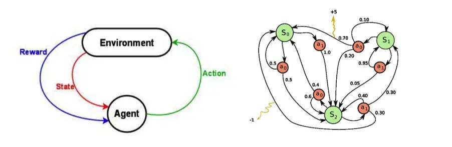
图 2:左:强化学习问题。右:Markov decision process

状态和行动的集合,以及从一个状态跳转到另一个状态的规则,共同真诚了 Markov decision process。这个过程(比方说一次游戏过程)的一个 episode 形成了一个有限的状态、行动和收益的序列:

这里的 s_i 表示状态,a_i 表示行动,而 r_{i+1} 是在执行行动的汇报。episode 以 terminal 状态 s_n 结尾(可能就是“游戏结束”画面)。MDP 依赖于 Markov 假设——下一个状态 s_{i+1} 的概率仅仅依赖于当前的状态 s_i 和行动 a_i,但不依赖此前的状态和行动。

Discounted Future Reward

To perform well in the long-term, we need to take into account not only the immediate rewards, but also the future rewards we are going to get. How should we go about that?

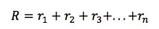
Given one run of the Markov decision process, we can easily calculate the total reward for one episode:

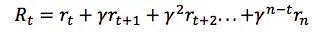
Given that, the total future reward from time point t onward can be expressed as:

But because our environment is stochastic, we can never be sure, if we will get the same rewards the next time we perform the same actions. The more into the future we go, the more it may diverge. For that reason it is common to use discounted future reward instead:

Here γ is the discount factor between 0 and 1 – the more into the future the reward is, the less we take it into consideration. It is easy to see, that discounted future reward at time step t can be expressed in terms of the same thing at time step t+1:

If we set the discount factor γ=0, then our strategy will be short-sighted and we rely only on the immediate rewards. If we want to balance between immediate and future rewards, we should set discount factor to something like γ=0.9. If our environment is deterministic and the same actions always result in same rewards, then we can set discount factor γ=1.

A good strategy for an agent would be to always choose an action that maximizes the (discounted) future reward.

Q-learning

In Q-learning we define a function Q(s, a) representing the maximum discounted future reward when we perform action a in state s, and continue optimally from that point on.

**

**The way to think about Q(s, a) is that it is “the best possible score at the end of the game after performing action a in state s“. It is called Q-function, because it represents the “quality” of a certain action in a given state.

This may sound like quite a puzzling definition. How can we estimate the score at the end of game, if we know just the current state and action, and not the actions and rewards coming after that? We really can’t. But as a theoretical construct we can assume existence of such a function. Just close your eyes and repeat to yourself five times: “Q(s, a) exists, Q(s, a) exists, …”. Feel it?

If you’re still not convinced, then consider what the implications of having such a function would be. Suppose you are in state and pondering whether you should take action a or b. You want to select the action that results in the highest score at the end of game. Once you have the magical Q-function, the answer becomes really simple – pick the action with the highest Q-value!

Here π represents the policy, the rule how we choose an action in each state.

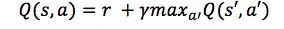
OK, how do we get that Q-function then? Let’s focus on just one transition <s, a, r, s’>. Just like with discounted future rewards in the previous section, we can express the Q-value of state s and action a in terms of the Q-value of the next state s’.

This is called the Bellman equation. If you think about it, it is quite logical – maximum future reward for this state and action is the immediate reward plus maximum future reward for the next state.

The main idea in Q-learning is that we can iteratively approximate the Q-function using the Bellman equation. In the simplest case the Q-function is implemented as a table, with states as rows and actions as columns. The gist of the Q-learning algorithm is as simple as the following[1]:

α in the algorithm is a learning rate that controls how much of the difference between previous Q-value and newly proposed Q-value is taken into account. In particular, when α=1, then two Q[s,a] cancel and the update is exactly the same as the Bellman equation.

The maxa’ Q[s’,a’] that we use to update Q[s,a] is only an approximation and in early stages of learning it may be completely wrong. However the approximation get more and more accurate with every iteration and it has been shown, that if we perform this update enough times, then the Q-function will converge and represent the true Q-value.

Deep Q Network

环境的状态可以用 paddle 的位置,球的位置和方向以及每个砖块是否消除来确定。不过这个直觉上的表示与游戏相关。我们能不能获得某种更加通用适合所有游戏的表示呢?最明显的选择就是屏幕像素——他们隐式地包含所有关于除了球的速度和方向外的游戏情形的相关信息。不过两个时间上相邻接的屏幕可以包含这两个丢失的信息。

如果我们像 DeepMind 的论文中那样处理游戏屏幕的话——获取四幅最后的屏幕画面,将他们重新规整为 84 X 84 的大小,转换为 256 灰度层级——我们会得到一个 256^{84X84X4} 大小的可能游戏状态。这意味着我们的 Q-table 中需要有 10^67970 行——这比已知的宇宙空间中的原子的数量还要大得多!可能有人会说,很多像素的组合(也就是状态)不会出现——这样其实可以使用一个稀疏的 table 来包含那些被访问到的状态。即使这样,很多的状态仍然是很少被访问到的,也许需要宇宙的生命这么长的时间让 Q-table 收敛。我们希望理想化的情形是有一个对那些还未遇见的状态的 Q-value 的猜测。

这里就是深度学习发挥作用的地方。神经网络其实对从高度结构化的数据中获取特征非常在行。我们可以用神经网络表示 Q-function,以状态(四幅屏幕画面)和行动作为输入,以对应的 Q-value 作为输出。另外,我们可以仅仅用游戏画面作为输入对每个可能的行动输出一个 Q-value。后面这个观点对于我们想要进行 Q-value 的更新或者选择最优的 Q-value 对应操作来说要更方便一些,这样我们仅仅需要进行一遍网络的前向传播就可立即得到所有行动的 Q-value。

图 3:左:DQN 的初级形式;右:DQN 的优化形式,用在 DeepMind 的论文中的版本

DeepMind 使用的深度神经网络架构如下:

这实际上是一个经典的卷积神经网络,包含 3 个卷积层加上 2 个全连接层。对图像识别的人们应该会注意到这里没有包含 pooling 层。但如果你好好想想这里的情况,你会明白,pooling 层会带来变换不变性 —— 网络会对图像中的对象的位置没有很强的感知。这个特性在诸如 ImageNet 这样的分类问题中会有用,但是在这里游戏的球的位置其实是潜在能够决定收益的关键因素,我们自然不希望失去这样的信息了!

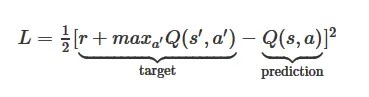
网络的输入是 4 幅 84X84 的灰度屏幕画面。网络的输出是对每个可能的行动(在 Atari 中是 18 个)。Q-value 可能是任何实数,其实这是一个回归任务,我们可以通过简单的平方误差来进行优化。

给定转移 <s, a, r, s’>,Q-table 更新规则变动如下:

  1. 对当前的状态 s 执行前向传播,获得对所有行动的预测 Q-value
  2. 对下一状态 s’ 执行前向传播,计算网络输出最大操作:max_{a’} Q(s’, a’)
  3. 设置行动的 Q-value 目标值为 r + γ max_{a’} Q(s’, a’)。使用第二步的 max 值。对所有其他的行动,设置为和第一步返回结果相同的 Q-value 目标值,让这些输出的误差设置为 0
  4. 使用反向传播算法更新权重

Experience Replay

到现在,我们有了使用 Q-learning 如何估计未来回报和用卷积神经网络近似 Q-function 的方法。但是有个问题是,使用非线性函数来近似 Q-value 其实是非常不稳定的。对这个问题其实也有一堆技巧来让其收敛。不过这样也会花点时间,在单个 GPU 上估计要一个礼拜。

其中最为重要的技巧是 experience replay。在游戏过程中,所有的经验 <s, a, r’, s’> 都存放在一个 replay memory 中。训练网络时,replay memory 中随机的 minibatch 会取代最近的状态转移。这会将连续的训练样本之间的相似性打破,否则容易将网络导向一个局部最优点。同样 experience replay 让训练任务与通常的监督学习更加相似,这样也简化了程序的 debug 和算法的测试。当然我们实际上也是可以收集人类玩家的 experience 并用这些数据进行训练。

Exploration-Exploitation

Q-learning 试着解决 credit assignment 问题——将受益按时间传播,直到导致获得受益的实际的关键决策点为止。但是我们并没有解决 exploration-exploitation 困境……

首先我们注意到,当 Q-table 或者 Q-network 随机初始化时,其预测结果也是随机的。如果我们选择一个拥有最高的 Q-value 的行动,这个行动是随机的,这样 agent 会进行任性的“exploration”。当 Q-function 收敛时,它会返回一个更加一致的 Q-value 此时 exploration 的次数就下降了。所以我们可以说,Q-learning 将 exploration 引入了算法的一部分。但是这样的 exploration 是贪心的,它会采用找到的最有效的策略。

对上面问题的一个简单却有效的解决方案是 ε-greedy exploration——以概率ε选择一个随机行动,否则按照最高的 Q-value 进行贪心行动。在 DeepMind 的系统中,对ε本身根据时间进行的从 1 到 0.1 的下降,也就是说开始时系统完全进行随机的行动来最大化地 explore 状态空间,然后逐渐下降到一个固定的 exploration 的比例。

Deep Q-learning 算法

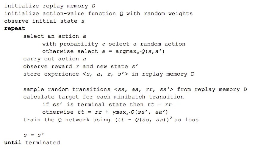
现在我们得到加入 experience replay的最终版本:

DeepMind 其实还使用了很多的技巧来让系统工作得更好——如 target network、error clipping、reward clipping 等等,这里我们不做介绍。

该算法最为有趣的一点就是它可以学习任何东西。你仔细想想——由于我们的 Q-function 是随机初始化的,刚开始给出的结果就完全是垃圾。然后我们就用这样的垃圾(下个状态的最高 Q-value)作为网络的目标,仅仅会偶然地引入微小的收益。这听起来非常疯狂,为什么它能够学习任何有意义的东西呢?然而,它确实如此神奇。

Final notes

Many improvements to deep Q-learning have been proposed since its first introduction – Double Q-learning, Prioritized Experience Replay, Dueling Network Architecture and extension to continuous action space to name a few. For latest advancements check out the NIPS 2015 deep reinforcement learning workshop and ICLR 2016 (search for “reinforcement” in title). But beware, that deep Q-learning has been patented by Google.

It is often said, that artificial intelligence is something we haven’t figured out yet. Once we know how it works, it doesn’t seem intelligent any more. But deep Q-networks still continue to amaze me. Watching them figure out a new game is like observing an animal in the wild – a rewarding experience by itself.

Credits

Thanks to Ardi Tampuu, Tanel Pärnamaa, Jaan Aru, Ilya Kuzovkin, Arjun Bansal and Urs Köster for comments and suggestions on the drafts of this post.

Links

David Silver’s lecture about deep reinforcement learning
Slightly awkward but accessible illustration of Q-learning
UC Berkley’s course on deep reinforcement learning
David Silver’s reinforcement learning course
Nando de Freitas’ course on machine learning (two lectures about reinforcement learning in the end)
Andrej Karpathy’s course on convolutional neural networks

[1] Algorithm adapted from http://artint.info/html/ArtInt_265.html


文/Not_GOD(简书作者)
原文链接:http://www.jianshu.com/p/d347bb2ca53c
著作权归作者所有,转载请联系作者获得授权,并标注“简书作者”。