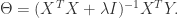
如果在某种特殊的情况下,特征的个数 n 大于样本的个数 m,i.e. 矩阵 X 的列数多于行数,那么 X 不是一个满秩矩阵,因此在计算 的时候会出现问题。为了解决这个问题,有人引入了岭回归(ridge regression)的概念。也就是说在计算矩阵的逆的时候,增加了一个对角矩阵,目的是使得可以对矩阵进行求逆。用数学语言来描述就是矩阵 加上 ,这里的 I 是一个 的对角矩阵,使得矩阵 是一个可逆矩阵。在这种情况下,回归系数的计算公式变成了
整个过程很像 Cross Validation。首先将训练数据分为 5 份,接下来一共 5 个迭代,每次迭代时,将 4 份数据作为 Training Set 对每个 Base Model 进行训练,然后在剩下一份 Hold-out Set 上进行预测。同时也要将其在测试数据上的预测保存下来。这样,每个 Base Model 在每次迭代时会对训练数据的其中 1 份做出预测,对测试数据的全部做出预测。5 个迭代都完成以后我们就获得了一个 #训练数据行数 x #Base Model 数量 的矩阵,这个矩阵接下来就作为第二层的 Model 的训练数据。当第二层的 Model 训练完以后,将之前保存的 Base Model 对测试数据的预测(因为每个 Base Model 被训练了 5 次,对测试数据的全体做了 5 次预测,所以对这 5 次求一个平均值,从而得到一个形状与第二层训练数据相同的矩阵)拿出来让它进行预测,就得到最后的输出。
Kaggle is the best place for learning from other data scientists. Many companies provide data and prize money to set up data science competitions on Kaggle. Recently I had my first shot on Kaggle and ranked 98th (~ 5%) among 2125 teams. Since this is my Kaggle debut, I feel quite satisfied. Because many Kaggle beginners set 10% as their first goal, here I want to share my experience in achieving that goal.
Most Kagglers use Python and R. I prefer Python, but R users should have no difficulty in understanding the ideas behind tools and languages.
First let’s go through some facts about Kaggle competitions in case you are not very familiar with them.
Different competitions have different tasks: classification, regression, recommendation, ordering… Training set and testing set will be open for download after the competition launches.
A competition typically lasts for 2 ~ 3 months. Each team can submit for a limited amount of times a day. Usually it’s 5 times a day.
There will be a deadline one week before the end of the competition, after which you cannot merge teams or enter the competition. Therefore be sure to have at least one valid submission before that.
You will get you score immediately after the submission. Different competitions use different scoring metrics, which are explained by the question mark on the leaderboard.
The score you get is calculated on a subset of testing set, which is commonly referred to as a Public LB score. Whereas the final result will use the remaining data in the testing set, which is referred to as Private LB score.
The score you get by local cross validation is commonly referred to as a CVscore. Generally speaking, CV scores are more reliable than LB scores.
Beginners can learn a lot from Forum and Scripts. Do not hesitate to ask, Kagglers are very kind and helpful.
I assume that readers are familiar with basic concepts and models of machine learning. Enjoy reading!
General Approach
In this section, I will walk you through the whole process of a Kaggle competition.
Data Exploration
What we do at this stage is called EDA (Exploratory Data Analysis), which means analytically exploring data in order to provide some insights for subsequent processing and modeling.
Usually we would load the data using Pandas and make some visualizations to understand the data.
Inspect the distribution of target variable. Depending on what scoring metric is used, an imbalanced distribution of target variable might harm the model’s performance.
For numerical variables, use box plot to inspect their distributions.
For coordinates-like data, use scatter plot to inspect the distribution and check for outliers.
For classification tasks, plot the data with points colored according to their labels. This can help with feature engineering.
Make pairwise distribution plots and examine correlations between pairs of variables.
We can perform some statistical tests to confirm our hypotheses. Sometimes we can get enough intuition from visualization, but quantitative results are always good to have. Note that we will always encounter non-i.i.d. data in real world. So we have to be careful about the choice of tests and how we interpret the findings.
In many competitions public LB scores are not very consistent with local CV scores due to noise or non-i.id. distribution. You can use test results to roughly set a threshold for determining whether an increase of score is an genuine one or due to randomness.
Data Preprocessing
In most cases, we need to preprocess the dataset before constructing features. Some common steps are:
Sometimes several files are provided and we need to join them.
Deal with noise. For example you may have some floats derived from unknown integers. The loss of precision during floating-point operations can bring much noise into the data: two seemingly different values might be the same before conversion. Sometimes noise harms model and we would want to avoid that.
How we choose to perform preprocessing largely depends on what we learn about the data in the previous stage. In practice, I recommend using iPython Notebook for data manipulating and mastering usages of frequently used Pandas operations. The advantage is that you get to see the results immediately and are able to modify or rerun operations. Also this makes it very convenient to share your approaches with others. After all reproducible results are very important in data science.
Let’s have some examples.
Outlier
The plot shows some scaled coordinates data. We can see that there are some outliers in the top-right corner. Exclude them and the distribution looks good.
Dummy Variables
For categorical variables, a common practice is One-hot Encoding. For a categorical variable with n possible values, we create a group of n dummy variables. Suppose a record in the data takes one value for this variable, then the corresponding dummy variable is set to 1 while other dummies in the same group are all set to 0.
Like this, we transform DayOfWeek into 7 dummy variables.
Note that when the categorical variable can takes many values (hundreds or more), this might not work well. It’s difficult to find a general solution to that, but I’ll discuss one scenario in the next section.
Feature Engineering
Some describe the essence of Kaggle competitions as feature engineering supplemented by model tuning and ensemble learning. Yes, that makes a lot of sense. Feature engineering gets your very far. Yet it is how well you know about the domain of given data that decides how far you can go. For example, in a competition where data is mainly consisted of texts, common NLP features are a must. The approach of constructing useful features is something we all have to continuously learn in order to do better.
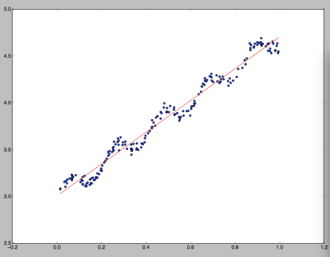
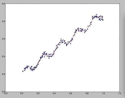
Basically, when you feel that a variable is intuitively useful for the task, you can include it as a feature. But how do you know it actually works? The simplest way is to check by plotting it against the target variable like this:
Feature Selection
Generally speaking, we should try to craft as many features as we can and have faith in the model’s ability to pick up the most significant features. Yet there’s still something to gain from feature selection beforehand:
Less features mean faster training
Some features are linearly related to others. This might put a strain on the model.
By picking up the most important features, we can use interactions between them as new features. Sometimes this gives surprising improvement.
The simplest way to inspect feature importance is by fitting a random forest model. There exist more robust feature selection algorithms (e.g. this) which are theoretically superior but not practicable due to the absence of efficient implementation. You can combat noisy data (to an extent) simply by increasing number of trees used in random forest.
This is important for competitions in which data is anonymized because you won’t waste time trying to figure out the meaning of a variable that’s of no significance.
Feature Encoding
Sometimes raw features have to be converted to some other formats for them to be work properly.
For example, suppose we have a categorical variable which can take more than 10K different values. Then naively creating dummy variables is not a feasible option. An acceptable solution is to create dummy variables for only a subset of the values (e.g. values that constitute 95% of the feature importance) and assign everything else to an ‘others’ class.
Model Selection
With the features set, we can start training models. Kaggle competitions usually favor tree-based models:
Gradient Boosted Trees
Random Forest
Extra Randomized Trees
These models are slightly worse in terms of performance, but are suitable as base models in ensemble learning (will be discussed later):
SVM
Linear Regression
Logistic Regression
Neural Networks
Of course, neural networks are very important in image-related competitions.
Here I want to emphasize the greatness of Xgboost. The outstanding performance of gradient boosted trees and Xgboost’s efficient implementation makes it very popular in Kaggle competitions. Nowadays almost every winner uses Xgboost in one way or another.
BTW, installing Xgboost on Windows could be a painstaking process. You can refer to this post by me if you run into problems.
Model Training
We can obtain a good model by tuning its parameters. A model usually have many parameters, but only a few of them are important to its performance. For example, the most important parameters for random forset is the number of trees in the forest and the maximum number of features used in developing each tree. We need to understand how models work and what impact does each of the parameters have to the model’s performance, be it accuracy, robustness or speed.
Normally we would find the best set of parameters by a process called grid search. Actually what it does is simply iterating through all the possible combinations and find the best one.
By the way, random forest usually reach optimum when max_features is set to the square root of the total number of features.
Here I’d like to stress some points about tuning XGB. These parameters are generally considered to have real impacts on its performance:
eta: Step size used in updating weights. Lower eta means slower training.
num_round: Total round of iterations.
subsample: The ratio of training data used in each iteration. This is to combat overfitting.
colsample_bytree: The ratio of features used in each iteration. This is like max_features of RandomForestClassifier.
max_depth: The maximum depth of each tree. Unlike random forest,gradient boosting would eventually overfit if we do not limit its depth.
early_stopping_rounds: Controls how many iterations that do not show a increase of score on validation set are needed for the algorithm to stop early. This is to combat overfitting, too.
Usual tuning steps:
Reserve a portion of training set as the validation set.
Set eta to a relatively high value (e.g. 0.1), num_round to 300 ~ 500.
Use grid search to find best combination of other parameters.
Gradually lower eta to find the optimum.
Use the validation set as watch_list to re-train the model with the best parameters. Observe how score changes on validation set in each iteration. Find the optimal value for early_stopping_rounds.
Finally, note that models with randomness all have a parameter like seed or random_state to control the random seed. You must record this with all other parameters when you get a good model. Otherwise you wouldn’t be able to reproduce it.
Cross Validation
Cross validation is an essential step. It tells us whether our model is at high risk of overfitting. In many competitions, public LB scores are not very reliable. Often when we improve the model and get a better local CV score, the LB score becomes worse. It is widely believed that we should trust our CV scores under such situation. Ideally we would want CV scores obtained by different approaches to improve in sync with each other and with the LB score, but this is not always possible.
Usually 5-fold CV is good enough. If we use more folds, the CV score would become more reliable, but the training takes longer to finish as well.
How to do CV properly is not a trivial problem. It requires constant experiment and case-by-case discussion. Many Kagglers share their CV approaches (like this one) after competitions where it’s not easy to do reliable CV.
Ensemble Generation
Ensemble Learning refers to ways of combining different models. It reduces both bias and variance of the final model (you can find a proof here), thusincreasing the score and reducing the risk of overfitting. Recently it became virtually impossible to win prize without using ensemble in Kaggle competitions.
Common approaches of ensemble learning are:
Bagging: Use different random subsets of training data to train each base model. Then base models vote to generate the final predictions. This is how random forest works.
Boosting: Train base models iteratively, modify the weights of training samples according to the last iteration. This is how gradient boosted trees work. It performs better than bagging but is more prone to overfitting.
Blending: Use non-overlapping data to train different base models and take a weighted average of them to obtain the final predictions. This is easy to implement but uses less data.
Stacking: To be discussed next.
In theory, for the ensemble to perform well, two elements matter:
Base models should be as unrelated as possibly. This is why we tend to include non-tree-base models in the ensemble even though they don’t perform as well. The math says that the greater the diversity, and less bias in the final ensemble.
Performance of base models shouldn’t differ to much.
Actually we have a trade-off here. In practice we may end up with highly related models of comparable performances. Yet we ensemble them anyway because it usually increase performance even under this circumstance.
Stacking
Compared with blending, stacking makes better use of training data. Here’s a diagram of how it works:
It’s much like cross validation. Take 5-fold stacking as an example. First we split the training data into 5 folds. Next we will do 5 iterations. In each iteration, train every base model on 4 folds and predict on the hold-out fold. You have to keep the predictions on the testing data as well. This way, in each iteration every base model will make predictions on 1 fold of the training data and all of the testing data. After 5 iterations we will obtain a matrix of shape #(rows in training data) X #(base models). This matrix is then fed to the stacker in the second level. After the stacker is fitted, use the predictions on testing data by base models (each base model is trained 5 times, therefore we have to take an average to obtain a matrix of the same shape) as the input for the stacker and obtain our final predictions.
Prize winners usually have larger and much more complicated ensembles. For beginner, implementing a correct 5-fold stacking is good enough.
*Pipeline
We can see that the workflow for a Kaggle competition is quite complex, especially for model selection and ensemble. Ideally, we need a highly automated pipeline capable of:
Modularized feature transform. We only need to write a few lines of codes and the new feature is added to the training set.
Automated grid search. We only need to set up models and parameter grid, the search will be run and best parameters are recorded.
Automated ensemble generation. Use best K models for ensemble as soon as last generation is done.
For beginners, the first one is not very important because the number of features is quite manageable; the third one is not important either because typically we only do several ensembles at the end of the competition. But the second one is good to have because manually recording the performance and parameters of each model is time-consuming and error-prone.
Chenglong Chen, the winner of Crowdflower Search Results Relevance, once released his pipeline on GitHub. It’s very complete and efficient. Yet it’s still very hard to understand and extract all his logic to build a general framework. This is something you might want to do when you have plenty of time.
Home Depot Search Relevance
In this section I will share my solution in Home Depot Search Relevance and what I learned from top teams after the competition.
The task in this competitions is to predict how relevant a result is for a search term on Home Depot website. The relevance score is an average of three human evaluators and ranges between 1 ~ 3. Therefore it’s a regression task. The datasets contains search terms, product titles / descriptions and some attributes like brand, size and color. The metric is RMSE.
This is much like Crowdflower Search Results Relevance. The difference is thatQuadratic Weighted Kappa is used in that competition and therefore complicated the final cutoff of regression scores. Also there were no attributes provided in that competition.
EDA
There were several quite good EDAs by the time I joined the competition, especially this one. I learned that:
Many search terms / products appeared several times.
Text similarities are great features.
Many products don’t have attributes features. Would this be a problem?
Product ID seems to have strong predictive power. However the overlap of product ID between the training set and the testing set is not very high. Would this contribute to overfitting?
Preprocessing
You can find how I did preprocessing and feature engineering on GitHub. I’ll only give a brief summary here:
Use typo dictionary posted in forum to correct typos in search terms.
Count attributes. Find those frequent and easily exploited ones.
Join the training set with the testing set. This is important because otherwise you’ll have to do feature transform twice.
Do stemming and tokenizing for all the text fields. Some normalization(with digits and units) and synonym substitutions are performed manually.
Feature
*Attribute Features
Whether the product contains a certain attribute (brand, size, color, weight, indoor/outdoor, energy star certified …)
Whether a certain attribute matches with search term
Meta Features
Length of each text field
Whether the product contains attribute fields
Brand (encoded as integers)
Product ID
Matching
Whether search term appears in product title / description / attributes
Count and ratio of search term’s appearance in product title / description / attributes
*Whether the i-th word of search term appears in product title / description / attributes
Text similarities between search term and product title/description/attributes
Word2Vec Distance (I didn’t include this because of poor performance. Yet it seems that I was using it wrong.)
Latent Semantic Indexing: By performing SVD decomposition to the matrix obtained from BOW/TF-IDF Vectorization, we get the latent descriptions of different search term / product groups. This enables our model to distinguish between groups and assign different weights to features, therefore solving the issue of dependent data and products lacking some features (to an extent).
Note that features listed above with * are the last batch of features I added. The problem is that the model trained on data that included these features performed worse than the previous ones. At first I thought that the increase in number of features would require re-tuning of model parameters. However, after wasting much CPU time on grid search, I still could not beat the old model. I think it might be the issue of feature correlation mentioned above. I actually knew a solution that might work, which is to combine models trained on different version of features by stacking. Unfortunately I didn’t have enough time to try it. As a matter of fact, most of top teams regard the ensemble of models trained with different preprocessing and feature engineering pipelines as a key to success.
Model
At first I was using RandomForestRegressor to build my model. Then I triedXgboost and it turned out to be more than twice as fast as Sklearn. From that on what I do everyday is basically running grid search on my PC while working on features on my laptop.
Dataset in this competition is not trivial to validate. It’s not i.i.d. and many records are dependent. Many times I used better features / parameters only to end with worse LB scores. As repeatedly stated by many accomplished Kagglers, you have to trust your own CV score under such situation. Therefore I decided to use 10-fold instead of 5-fold in cross validation and ignore the LB score in the following attempts.
Ensemble
My final model is an ensemble consisting of 4 base models:
RandomForestRegressor
ExtraTreesRegressor
GradientBoostingRegressor
XGBRegressor
The stacker (L2 model) is also a XGBRegressor.
The problem is that all my base models are highly correlated (with a lowest correlation of 0.9). I thought of including linear regression, SVM regression and XGBRegressor with linear booster into the ensemble, but these models had RMSE scores that are 0.02 higher (this accounts for a gap of hundreds of places on the leaderboard) than the 4 models I finally used. Therefore I decided not to use more models although they would have brought much more diversity.
The good news is that, despite base models being highly correlated, stacking really bumps up my score. What’s more, my CV score and LB score are in complete sync after I started stacking.
During the last two days of the competition, I did one more thing: use 20 or so different random seeds to generate the ensemble and take a weighted average of them as the final submission. This is actually a kind of bagging. It makes sense in theory because in stacking I used 80% of the data to train base models in each iteration, whereas 100% of the data is used to train the stacker. Therefore it’s less clean. Making multiple runs with different seeds makes sure that different 80% of the data are used each time, thus reducing the risk of information leak. Yet by doing this I only achieved an increase of 0.0004, which might be just due to randomness.
After the competition, I found out that my best single model scores 0.46378 on the private leaderboard, whereas my best stacking ensemble scores 0.45849. That was the difference between the 174th place and the 98th place. In other words, feature engineering and model tuning got me into 10%, whereas stacking got me into 5%.
Lessons Learned
There’s much to learn from the solutions shared by top teams:
There’s a pattern in the product title. For example, whether a product is accompanied by a certain accessory will be indicated by With/Without XXXat the end of the title.
Some features based on letters instead of words. At first I was rather confused by this. But it makes perfect sense if you consider it. For example, the team that won the 3rd place took the number of letters matched into consideration when computing text similarity. They argued that longer words are more specific and thus more likely to be assigned high relevance scores by human. They also used char-by-char sequence comparison (difflib.SequenceMatcher) to measure visual similarity, which they claimed to be important for human.
POS-tag words and find anchor words. Use anchor words for computing various distances.
Extract top-ranking trigrams from the TF-IDF of product title / description field and compute the ratio of word from search terms that appear in these trigrams. Vice versa. This is like computing latent indexes from another point of view.
Generate pairwise polynomial interactions between top-ranking features.
For CV, construct splits in which product IDs do not overlap between training set and testing set, and splits in which IDs do. Then we can use these with corresponding ratio to approximate the impact of public/private LB split in our local CV.
Summary
Takeaways
It was a good call to start doing ensembles early in the competition. As it turned out, I was still playing with features during the very last days.
It’s of high priority that I build a pipeline capable of automatic model training and recording best parameters.
Features matter the most! I didn’t spend enough time on features in this competition.
If possible, spend some time to manually inspect raw data for patterns.
Issues Raised
Several issues I encountered in this competitions are of high research values.
How to do reliable CV with dependent data.
How to quantify the trade-off between diversity and accuracy in ensemble learning.
How to deal with feature interaction which harms the model’s performance. And how to determine whether new features are effective in such situation.
Beginner Tips
Choose a competition you’re interested in. It would be better if you’ve already have some insights about the problem domain.
Following my approach or somebody else’s, start exploring, understanding and modeling data.
Learn from forum and scripts. See how other interpret data and construct features.
Find winner interviews / blog post of previous competitions. They’re very helpful.
Start doing ensemble after you have reached a pretty good score (e.g. ~ 10%) or you feel that there isn’t much room for new features (which, sadly, always turns out to be false).
If you think you may have a chance to win the prize, try teaming up!
Don’t give up until the end of the competition. At least try something new every day.
Learn from the sharings of top teams after the competition. Reflect on your approaches. If possible, spend some time verifying what you learn.
Exabeam并没有固守昔日的防御策略,而是基于Gartner的UBA( User Behavior Analytics,用户行为分析)概念采取了主动出击的方法。UBA背后的思路是你没法事先知道机器或用户的好坏,所以先假设他们是恶意的,你的网络是缺乏抵抗力的,所以你时刻对每个人的行为进行监测和制作模型,从而找到恶意行为者。
You’re sitting at home minding your own business when you get a call from your credit card’s fraud detection unit asking if you’ve just made a purchase at a department store in your city. It wasn’t you who bought expensive electronics using your credit card – in fact, it’s been in your pocket all afternoon. So how did the bank know to flag this single purchase as most likely fraudulent?
Credit card companies have a vested interest in identifying financial transactions that are illegitimate and criminal in nature. The stakes are high. According to the Federal Reserve Payments Study, Americans used credit cards to pay for 26.2 billion purchases in 2012. The estimated loss due to unauthorized transactions that year was US$6.1 billion. The federal Fair Credit Billing Act limits the maximum liability of a credit card owner to $50 for unauthorized transactions, leaving credit card companies on the hook for the balance. Obviously fraudulent payments can have a big effect on the companies’ bottom lines. The industry requires any vendors that process credit cards to go through security audits every year. But that doesn’t stop all fraud.
In the banking industry, measuring risk is critical. The overall goal is to figure out what’s fraudulent and what’s not as quickly as possible, before too much financial damage has been done. So how does it all work? And who’s winning in the arms race between the thieves and the financial institutions?
Gathering the troops
From the consumer perspective, fraud detection can seem magical. The process appears instantaneous, with no human beings in sight. This apparently seamless and instant action involves a number of sophisticated technologies in areas ranging from finance and economics to law to information sciences.
Of course, there are some relatively straightforward and simple detection mechanisms that don’t require advanced reasoning. For example, one good indicator of fraud can be an inability to provide the correct zip code affiliated with a credit card when it’s used at an unusual location. But fraudsters are adept at bypassing this kind of routine check – after all, finding out a victim’s zip code could be as simple as doing a Google search.
Traditionally, detecting fraud relied on data analysis techniques that required significant human involvement. An algorithm would flag suspicious cases to be closely reviewed ultimately by human investigators who may even have called the affected cardholders to ask if they’d actually made the charges. Nowadays the companies are dealing with a constant deluge of so many transactions that they need to rely on big data analytics for help. Emerging technologies such as machine learning and cloud computing are stepping up the detection game.
Learning what’s legit, what’s shady
Simply put, machine learning refers to self-improving algorithms, which are predefined processes conforming to specific rules, performed by a computer. A computer starts with a model and then trains it through trial and error. It can then make predictions such as the risks associated with a financial transaction.
A machine learning algorithm for fraud detection needs to be trained first by being fed the normal transaction data of lots and lots of cardholders. Transaction sequences are an example of this kind of training data. A person may typically pump gas one time a week, go grocery shopping every two weeks and so on. The algorithm learns that this is a normal transaction sequence.
After this fine-tuning process, credit card transactions are run through the algorithm, ideally in real time. It then produces a probability number indicating the possibility of a transaction being fraudulent (for instance, 97%). If the fraud detection system is configured to block any transactions whose score is above, say, 95%, this assessment could immediately trigger a card rejection at the point of sale.
The algorithm considers many factors to qualify a transaction as fraudulent: trustworthiness of the vendor, a cardholder’s purchasing behavior including time and location, IP addresses, etc. The more data points there are, the more accurate the decision becomes.
This process makes just-in-time or real-time fraud detection possible. No person can evaluate thousands of data points simultaneously and make a decision in a split second.
Here’s a typical scenario. When you go to a cashier to check out at the grocery store, you swipe your card. Transaction details such as time stamp, amount, merchant identifier and membership tenure go to the card issuer. These data are fed to the algorithm that’s learned your purchasing patterns. Does this particular transaction fit your behavioral profile, consisting of many historic purchasing scenarios and data points?
The algorithm knows right away if your card is being used at the restaurant you go to every Saturday morning – or at a gas station two time zones away at an odd time such as 3:00 a.m. It also checks if your transaction sequence is out of the ordinary. If the card is suddenly used for cash-advance services twice on the same day when the historic data show no such use, this behavior is going to up the fraud probability score. If the transaction’s fraud score is above a certain threshold, often after a quick human review, the algorithm will communicate with the point-of-sale system and ask it to reject the transaction. Online purchases go through the same process.
In this type of system, heavy human interventions are becoming a thing of the past. In fact, they could actually be in the way since the reaction time will be much longer if a human being is too heavily involved in the fraud-detection cycle. However, people can still play a role – either when validating a fraud or following up with a rejected transaction. When a card is being denied for multiple transactions, a person can call the cardholder before canceling the card permanently.
Computer detectives, in the cloud
The sheer number of financial transactions to process is overwhelming, truly, in the realm of big data. But machine learning thrives on mountains of data – more information actually increases the accuracy of the algorithm, helping to eliminate false positives. These can be triggered by suspicious transactions that are really legitimate (for instance, a card used at an unexpected location). Too many alerts are as bad as none at all.
It takes a lot of computing power to churn through this volume of data. For instance, PayPal processes more than 1.1 petabytes of data for 169 million customer accounts at any given moment. This abundance of data – one petabyte, for instance, is more than 200,000 DVDs’ worth – has a positive influence on the algorithms’ machine learning, but can also be a burden on an organization’s computing infrastructure.
Enter cloud computing. Off-site computing resources can play an important role here. Cloud computing is scalable and not limited by the company’s own computing power.
Fraud detection is an arms race between good guys and bad guys. At the moment, the good guys seem to be gaining ground, with emerging innovations in IT technologies such as chip and pin technologies, combined with encryption capabilities, machine learning, big data and, of course, cloud computing.
Fraudsters will surely continue trying to outwit the good guys and challenge the limits of the fraud detection system. Drastic changes in the payment paradigms themselves are another hurdle. Your phone is now capable of storing credit card information and can be used to make payments wirelessly – introducing new vulnerabilities. Luckily, the current generation of fraud detection technology is largely neutral to the payment system technologies.
One of our weapons in the fight against spam, malware, and other abuse on Facebook is a system called Sigma. Its job is to proactively identify malicious actions on Facebook, such as spam, phishing attacks, posting links to malware, etc. Bad content detected by Sigma is removed automatically so that it doesn’t show up in your News Feed.
We recently completed a two-year-long major redesign of Sigma, which involved replacing the in-house FXL language previously used to program Sigma with Haskell. The Haskell-powered Sigma now runs in production, serving more than one million requests per second.
Haskell isn’t a common choice for large production systems like Sigma, and in this post, we’ll explain some of the thinking that led to that decision. We also wanted to share the experiences and lessons we learned along the way. We made several improvements to GHC (the Haskell compiler) and fed them back upstream, and we were able to achieve better performance from Haskell compared with the previous implementation.
How does Sigma work?
Sigma is a rule engine, which means it runs a set of rules, called policies. Every interaction on Facebook — from posting a status update to clicking “like” — results in Sigma evaluating a set of policies specific to that type of interaction. These policies make it possible for us to identify and block malicious interactions before they affect people on Facebook.
Policies are continuously deployed. At all times, the source code in the repository is the code running in Sigma, allowing us to move quickly to deploy policies in response to new abuses. This also means that safety in the language we write policies in is important. We don’t allow code to be checked into the repository unless it is type-correct.
Louis Brandy of Facebook’s Site Integrity team discusses scalable spam fighting and the anti-abuse structure at Facebook and Instagram in a 2014 @Scale talk.
Why Haskell?
The original language we designed for writing policies, FXL, was not ideal for expressing the growing scale and complexity of Facebook policies. It lacked certain abstraction facilities, such as user-defined data types and modules, and its implementation, based on an interpreter, was slower than we wanted. We wanted the performance and expressivity of a fully fledged programming language. Thus, we decided to migrate to an existing language rather than try to improve FXL.
The following features were at the top of our list when we were choosing a replacement:
1. Purely functional and strongly typed. This ensures that policies can’t inadvertently interact with each other, they can’t crash Sigma, and they are easy to test in isolation. Strong types help eliminate many bugs before putting policies into production.
2. Automatically batch and overlap data fetches. Policies typically fetch data from other systems at Facebook, so we want to employ concurrency wherever possible for efficiency. We want concurrency to be implicit, so that engineers writing policies can concentrate on fighting spam and not worry about concurrency. Implicit concurrency also prevents the code from being cluttered with efficiency-related details that would obscure the functionality, and make the code harder to understand and modify.
3. Push code changes to production in minutes. This enables us to deploy new or updated policies quickly.
4. Performance. FXL’s slower performance meant that we were writing anything performance-critical in C++ and putting it in Sigma itself. This had a number of drawbacks, particularly the time required to roll out changes.
5. Support for interactive development. Developers working on policies want to be able to experiment and test their code interactively, and to see the results immediately.
Haskell measures up quite well: It is a purely functional and strongly typed language, and it has a mature optimizing compiler and an interactive environment (GHCi). It also has all the abstraction facilities we would need, it has a rich set of libraries available, and it’s backed by an active developer community.
That left us with two features from our list to address: (1) automatic batching and concurrency, and (2) hot-swapping of compiled code.
Automatic batching and concurrency: The Haxl framework
All the existing concurrency abstractions in Haskell are explicit, meaning that the user needs to say which things should happen concurrently. For data-fetching, which can be considered a purely functional operation, we wanted a programming model in which the system just exploits whatever concurrency is available, without the programmer having to use explicit concurrency constructs. We developed the Haxl framework to address this issue: Haxl enables multiple data-fetching operations to be automatically batched and executed concurrently.
In addition to the Haxl framework, we needed help from the Haskell compiler in the form of theApplicative do-notation. This allows programmers to write sequences of statements that the compiler automatically rearranges to exploit concurrency. We also designed and implemented Applicative do-notation in GHC.
Hot-swapping of compiled code
Every time someone checks new code into the repository of policies, we want to have that code running on every machine in the Sigma fleet as quickly as possible. Haskell is a compiled language, so that involves compiling the code and distributing the new compiled code to all the machines running Sigma.
We want to update the compiled rules in a running Sigma process on the fly, while it is serving requests. Changing the code of a running program is a tricky problem in general, and it has been the subject of a great deal of research in the academic community. In our case, fortunately, the problem is simpler: Requests to Sigma are short-lived, so we don’t need to switch a running request to new code. We can serve new requests on the new code and let the existing requests finish before we discard the old code. We’re careful to ensure that we don’t change any code associated with persistent state in Sigma.
Loading and unloading code currently uses GHC’s built-in runtime linker, although in principle, we could use the system dynamic linker. To unload the old version of the code, the garbage collector gets involved. The garbage collector detects when old code is no longer being used by a running request, so we know when it is safe to unload it from the running process.
How Haskell fits in
Haskell is sandwiched between two layers of C++ in Sigma. At the top, we use the C++ thrift server. In principle, Haskell can act as a thrift server, but the C++ thrift server is more mature and performant. It also supports more features. Furthermore, it can work seamlessly with the Haskell layers below because we can call into Haskell from C++. For these reasons, it made sense to use C++ for the server layer.
At the lowest layer, we have existing C++ client code for talking to other internal services. Rather than rewrite this code in Haskell, which would duplicate the functionality and create an additional maintenance burden, we wrapped each C++ client in a Haxl data source using Haskell’s Foreign Function Interface (FFI) so we could use it from Haskell.
Haskell’s FFI is designed to call C rather than C++, so calling C++ requires an intermediate C layer. In most cases, we were able to avoid the intermediate C layer by using a compile-time tool that demangles C++ function names so they can be called directly from Haskell.
Performance
Perhaps the biggest question here is “Does it run fast enough?” Requests to Sigma result from users performing actions on Facebook, such as sending a message on Messenger, and Sigma must respond before the action can take place. So we wanted to serve requests fast enough to avoid interruptions to the user experience.
The graph below shows the relative throughput performance between FXL and Haskell for the 25 most common types of requests served by Sigma (these requests account for approximately 95 percent of Sigma’s typical workload).
Haskell performs as much as three times faster than FXL for certain requests. On a typical workload mix, we measured a 20 percent to 30 percent improvement in overall throughput, meaning we can serve 20 percent to 30 percent more traffic with the same hardware. We believe additional improvements are possible through performance analysis, tuning, and optimizing the GHC runtime for our workload.
Achieving this level of performance required a lot of hard work, profiling the Haskell code, and identifying and resolving performance bottlenecks.
Here are a few specific things we did:
We implemented automatic memoization of top-level computations using a source-to-source translator. This is particularly beneficial in our use-case where multiple policies can refer to the same shared value, and we want to compute it only once. Note, this is per-request memoization rather than global memoization, which lazy evaluation already provides.
We made a change to the way GHC manages the heap, to reduce the frequency of garbage collections on multicore machines. GHC’s default heap settings are frugal, so we also use a larger allocation area size of at least 64 MB per core.
Fetching remote data usually involves marshaling the data structure across the C++/Haskell boundary. If the whole data structure isn’t required, it is better to marshal only the pieces needed. Or better still, don’t fetch the whole thing — although that’s only possible if the remote service implements an appropriate API.
We uncovered a nasty performance bug in aeson, the Haskell JSON parsing library. Bryan O’Sullivan, the author of aeson, wrote a nice blog post about how he fixed it. It turns out that when you do things at Facebook scale, those one-in-a-million corner cases tend to crop up all the time.
Resource limits
In a latency-sensitive service, you don’t want a single request using a lot of resources and slowing down other requests on the same machine. In this case, the “resources” include everything on the machine that is shared by the running requests — CPU, memory, network bandwidth, and so on.
A request that uses a lot of resources is normally a bug that we want to fix. It does happen from time to time, often as a result of a condition that occurs in production that wasn’t encountered during testing — perhaps an innocuous operation provided with some unexpectedly large input data, or pathological performance of an algorithm on certain rare inputs, for example. When this happens, we want Sigma to terminate the affected request with an error (that will subsequently result in the bug being fixed) and continue without any impact on the performance of other requests being served.
To make this possible, we implemented allocation limits in GHC, which places a bound on the amount of memory a thread can allocate before it is terminated. Terminating a computation safely is a hard problem in general, but Haskell provides a safe way to abort a computation in the form of asynchronous exceptions. Asynchronous exceptions allow us to write most of most of our code ignoring the potential for summary termination and still have all the nice guarantees that we need in the event that the limit is hit, including safe releasing of resources, closing network connections, and so forth.
The following graph illustrates of how well allocation limits work in practice. It tracks the maximum live memory across various groups of machines in the Sigma fleet. When we enabled one request that had some resource-intensive outliers, we saw large spikes in the maximum live memory, which disappeared when we enabled allocation limits.
Enabling interactive development
Facebook engineers develop policies interactively, testing code against real data as they go. To enable this workflow in Haskell, we needed the GHCi environment to work with our full stack, including making requests to other back-end services from the command line.
To make this work, we had to make our build system link all the C++ dependencies of our code into a shared library that GHCi could load. We also customized the GHCi front end to implement some of our own commands and streamline the desired workflows. The result is an interactive environment in which developers can load their code from source in a few seconds and work on it with a fast turnaround time. They have the full set of APIs available and can test against real production data sources.
While GHCi isn’t as easy to customize as it could be, we’ve already made several improvements and contributed them upstream. We hope to make more improvements in the future.
Packages and build systems
In addition to GHC itself, we make use of a lot of open-source Haskell library code. Haskell has its own packaging and build system, Cabal, and the open-source packages are all hosted onHackage. The problem with this setup is that the pace of change on Hackage is fast, there are often breakages, and not all combinations of packages work well together. The system of version dependencies in Cabal relies too much on package authors getting it right, which is hard to ensure, and the tool support isn’t what it could be. We found that using packages directly from Hackage together with Facebook’s internal build tools meant adding or updating an existing package sometimes led to a yak-shaving exercise involving a cascade of updates to other packages, often with an element of trial and error to find the right version combinations.
As a result of this experience, we switched to Stackage as our source of packages. Stackage provides a set of package versions that are known to work together, freeing us from the problem of having to find the set by trial and error.
Did we find bugs in GHC?
Yes, most notably:
We fixed a bug in GHC’s garbage collector that was causing our Sigma processes to crash every few hours. The bug had gone undetected in GHC for several years.
We fixed a bug in GHC’s handling of finalizers that occasionally caused crashes during process shutdown.
Following these fixes, we haven’t seen any crashes in either the Haskell runtime or the Haskell code itself across our whole fleet.
What else?
At Facebook, we’re using Haskell at scale to fight spam and other types of abuse. We’ve found it to be reliable and performant in practice. Using the Haxl framework, our engineers working on spam fighting can focus on functionality rather than on performance, while the system can exploit the available concurrency automatically.
For more information on spam fighting at Facebook, check out our Protect the Graph page, or watch videos from our recent Spam Fighting @Scale event.
At the 2016 RSA Conference, you would be hard pressed to find a company that is not claiming to use ML for security. And why not? To the layperson, ML seems like the magic solution to all security problems. Take a bunch of unlabeled data, pump it through a system with some ML magic inside, and it can somehow identify patterns even human experts can’t find — all while learning and adapting to new behaviors and threats. Rather than having to code the rules, these systems can discover the rules all by themselves.
Oh, if only that were the case! ML is this year’s “big data”: Everyone is claiming to do it, but few actually do it right or even understand what it’s good for. Especially in security, I’ve seen more misapplications than appropriate ones.
Most applications of ML in security use a form of anomaly detection, which is used to spot events that do not match an expected pattern. Anomaly detection is a useful technique in certain circumstances, but too often, vendors misapply it. For example, they will claim to analyze network traffic in an enterprise and use ML to find hackers in your network. This does not work, and you should be immediately skeptical of the vendors who make this claim.
Effective machine learning requires a low dimensionality problem with high-quality labeled data. Unfortunately, deployments in real enterprises have neither. Detecting novel attacks requires either clear, labeled examples of attacks, which you do not have by definition, or a complete, exhaustive understanding of “normal” network behavior, which is impossible for any real network. And any sophisticated attacker will make an attack appear as seamless and “typical” as possible, to avoid setting off alarms.
Where does ML work?
One example where ML and anomaly detection can actually work well for security is in classifying human behavior. Humans, it turns out, are fairly predictable, and it is possible to build fairly accurate models of individual user behavior and detect when it doesn’t match their normal behavior.
We’ve had success in using ML for implicit authentication via analyzing a user’s biometrics, behavior, and environment. Implicit authentication is a technique that allows users to authenticate without performing any explicit actions like entering a password or swiping a fingerprint. This has clear benefits to both the user experience as well as for security. Users don’t need to be bothered with extra steps, we can use many authentication factors (rather than just one, a password), and it can happen continuously in the background.
Implicit authentication is well-suited to ML because most of the factors are low dimensional, meaning they involve a small number of parameters, and you can passively gather high-quality labeled data about user identities. Much like ML is effective in matching images for computer vision even in the presence of variance and noise, it is also effective in matching unique human behavioral aspects.
One example of this technology is how we can authenticate users based on unique aspects to the way they move. Attributes of the way you walk, sit, and stand are influenced by a large number of factors (including physiology, age, gender, and muscle memory), but are largely consistent for an individual. It is actually possible to accurately detect some of these attributes from the motion sensors in your phone in your pocket. In fact, after four seconds of motion data from a phone in your pocket, we can detect enough of these attributes to identify you. Another example is in using a user’s location history to authenticate them. Humans are creatures of habit, and by looking at where they came from and when, we can make an estimate of whether it’s them.
There are enough sensors in phones and computers (and more recently, wearables and IoT devices) that it is possible to passively pick up a large number of unique attributes about a user’s behavior and environment. We can then use ML to build a unique model for an individual user and find correlations between factors.
Threat models and anomaly detection
In any security system, it is important to understand the threat models you are trying to protect against. When using ML for security, you need to explicitly gather data, model the threats your system is protecting against, and use the model to train your system. Fortunately, for attacks against authentication, it is often possible to detect behavioral changes. For example, when a device is stolen, there are often clear changes in terms of its movement, location, and usage. And because false negatives are acceptable in that they just require the user to re-authenticate with a different method, we can tune the system to minimize false positives. In fact, once we combine four factors across multiple devices, we can get below a 0.001 percent false positive rate on implicit authentication.
There is no magic machine learning genie that can solve all your security problems. Building an effective security product that uses ML requires a deep understanding of the underlying system, and many security problems are just not appropriate for ML. For those that are, it’s a very powerful technique. And don’t worry, the companies on the hype train will soon move on to newer fads, like mobile self-driving AR blockchain drone marketplaces.
In this paper, we obtain the explicit value of the Hausdorff dimension of the graphs of the classical Weierstrass functions, by proving absolute continuity of the SRB measures of the associated solenoidal attractors.
Weierstrass (1872) and Hardy (1916) were interested in because they are concrete examples of continuous but nowhere differentiable functions.
Remark 1The graph of tends to be a “fractal object” because is self-similar in the sense that
We will come back to this point later.
Remark 2 is a -function for all . In fact, for all , we have
so that
whenever , i.e., .
The study of the graphs of as fractal sets started with the work of Besicovitch-Ursell in 1937.
Remark 3The Hausdorff dimension of the graph of a -function is
Indeed, for each , the Hölder continuity condition
leads us to the “natural cover” of by the family of rectangles given by
Nevertheless, a direct calculation with the family does not give us an appropriate bound on . In fact, since for each , we have
for . Because is arbitrary, we deduce that . Of course, this bound is certainly suboptimal for (because we know that anyway).Fortunately, we can refine the covering by taking into account that each rectangle tends to be more vertical than horizontal (i.e., its height is usually larger than its width ). More precisely, we can divide each rectangle into squares, say
such that every square has diameter . In this way, we obtain a covering of such that
for . Since is arbitrary, we conclude the desired bound
A long-standing conjecture about the fractal geometry of is:
Conjecture (Mandelbrot 1977): The Hausdorff dimension of the graph of is
Remark 4In view of remarks 2 and 3, the whole point of Mandelbrot’s conjecture is to establish the lower bound
Remark 5The analog of Mandelbrot conjecture for the box and packing dimensions is known to be true: see, e.g., these papers here and here).
In a recent paper (see here), Shen proved the following result:
Theorem 1 (Shen)For any integer and for all , the Mandelbrot conjecture is true, i.e.,
Remark 6The techniques employed by Shen also allow him to show that given a -periodic, non-constant, function, and given integer, there exists such that
for all .
Remark 7A previous important result towards Mandelbrot’s conjecture was obtained by Barańsky-Barány-Romanowska (in 2014): they proved that for all integer, there exists such that
for all .
The remainder of this post is dedicated to give some ideas of Shen’s proof of Theorem1 by discussing the particular case when and is large.
2. Ledrappier’s dynamical approach
If is an integer, then the self-similar function (cf. Remark 1) is also -periodic, i.e., for all . In particular, if is an integer, then is an invariant repeller for the endomorphism given by
This dynamical characterization of led Ledrappier to the following criterion for the validity of Mandelbrot’s conjecture when is an integer.
Denote by the alphabet . The unstable manifolds of through have slopes of the form
where , , , and
In this context, the push-forwards of the Bernoulli measure on (induced by the discrete measure assigning weight to each letter of the alphabet ) play the role of conditional measures along vertical fibers of the unique Sinai-Ruelle-Bowen (SRB) measure of the expanding endomorphism ,
where and . In plain terms, this means that
where is the unique -invariant probability measure which is absolutely continuous along unstable manifolds (see Tsujii’s paper).
As it was shown by Ledrappier in 1992, the fractal geometry of the conditional measures have important consequences for the fractal geometry of the graph :
Theorem 2 (Ledrappier)Suppose that for Lebesgue almost every the conditional measures have dimension , i.e.,
Then, the graph has Hausdorff dimension
Remark 8Very roughly speaking, the proof of Ledrappier theorem goes as follows. By Remark 4, it suffices to prove that . By Frostman lemma, we need to construct a Borel measure supported on such that
where . Finally, the main point is that the assumptions in Ledrappier theorem allow to prove that the measure given by the lift to of the Lebesgue measure on via the map satisfies
An interesting consequence of Ledrappier theorem and the equation 1 is the following criterion for Mandelbrot’s conjecture:
Corollary 3If is absolutely continuous with respect to the Lebesgue measure , then
Proof: By (1), the absolute continuity of implies that is absolutely continuous with respect to for Lebesgue almost every .
Since for almost every implies that for almost every , the desired corollary now follows from Ledrappier’s theorem.
3. Tsujii’s theorem
The relevance of Corollary 3 is explained by the fact that Tsujii found an explicittransversality condition implying the absolute continuity of .
More precisely, Tsujii firstly introduced the following definition:
Definition 4
Given , and , we say that two infinite words are -transverse at if either
or
Given , , and , we say that two finite words are -transverse at if , are -transverse at for all pairs of infinite words ; otherwise, we say that and are-tangent at ;
;
.
Next, Tsujii proves the following result:
Theorem 5 (Tsujii)If there exists integer such that , then
Remark 9Intuitively, Tsujii’s theorem says the following. The transversality condition implies that the majority of strong unstable manifolds are mutually transverse, so that they almost fill a small neighborhood of some point (see the figure below extracted from this paper of Tsujii). Since the SRB measure is absolutely continuous along strong unstable manifolds, the fact that the ‘s almost fill implies that becomes “comparable” to the restriction of the Lebesgue measure to .
Remark 10In this setting, Barańsky-Barány-Romanowska obtained their main result by showing that, for adequate choices of the parameters and , one has . Indeed, once we know that , since , they can apply Tsujii’s theorem and Ledrappier’s theorem (or rather Corollary 3) to derive the validity of Mandelbrot’s conjecture for certain parameters and .
For the sake of exposition, we will give just a flavor of the proof of Theorem 1 by sketching the derivation of the following result:
Proposition 6Let . If and is sufficiently large, then
In particular, by Corollary 3 and Tsujii’s theorem, if and is sufficiently large, then Mandelbrot’s conjecture is valid, i.e.,
Remark 11The proof of Theorem 1 in full generality (i.e., for integer and ) requires the introduction of a modified version of Tsujii’s transversality condition: roughly speaking, Shen defines a function (inspired from Peter-Paul inequality) and he proves
(a) a variant of Proposition 6: if integer and , then for some integer ;
(b) a variant of Tsujii’s theorem: if for some integer , then .
See Sections 2, 3, 4 and 5 of Shen’s paper for more details.
We start the (sketch of) proof of Proposition 6 by recalling that the slopes of unstable manifolds are given by
for , , so that
Remark 12Since , the series defining converges faster than the series defining .
By studying the first term of the expansion of and (while treating the remaining terms as a “small error term”), it is possible to show that if , then
and
(cf. Lemma 3.2 in Shen’s paper).
Using these estimates, we can find an upper bound for as follows. Take with , and let be such that distinct elements listed in such a way that


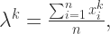
 ,假设其概率密度函数是
  ,它与一个未知参数
  相关。我们可以从这个分布中抽取
  样本
样本  ,我们就可以得到这个概率是
 .
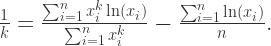
. ,然后利用这些数据来估算
  ,
, 的一阶导数等于零。这个使得
  称为
称为  个学生没有自行车,那么
  ; 否则
; 否则  . 并且假设
  的 Bernoulli 分布的。我们此时的目标是计算最大似然估计
  是相互独立的 Bernoulli 随机变量,那么对每一个
  .
. 可以定义为:
 .
. 求导:
求导:

 ,可以得到
,可以得到 .
. .
. 和
和  都是未知的。目标是寻找均值
  是满足正态分布的,那么对于每一个变量
  .
.


 和
和  ,可以求解方程组得到:
 ,
, .
.
 是 shape parameter。特别地,当
  时,Weibull 分布就是指数分布;当
  时,Weibull 分布就是 Rayleigh 分布。
 ,
, .
. .
. 那么对于每一个
  .
.


 的最大似然估计。第二个式子是关于
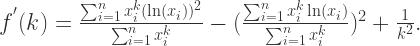

 ,换言之,
,换言之, 是关于
是关于 

 。如果从一个比较大的数开始的时候,可能使用 Newton 法的时候,会与负轴相交。但是如果从一个较小的数开始,就必定只与正数轴相交。其中 Newton 法的公式是:

 就可以被当作最大似然估计。
 = \sum\limits_{n=0}^{\infty} \lambda^n \cos(2\pi b^n x)")
 .
. = \sum\limits_{n=0}^{\infty} \lambda^n \phi(b^n x)")
 is a
is a  -periodic
  -function.
 because they are concrete examples of continuous but nowhere differentiable functions.
 tends to be a “fractal object” because
  = \phi(x) + \lambda f^{\phi}_{\lambda,b}(bx)")
 -function for all
  . In fact, for all
 ![{x,y\in[0,1]}](https://s0.wp.com/latex.php?latex=%7Bx%2Cy%5Cin%5B0%2C1%5D%7D&bg=ffffff&fg=000000&s=0 "{x,y\in[0,1]}") , we have
, we have - f^{\phi}_{\lambda,b}(y)}{|x-y|^{\alpha}} = \sum\limits_{n=0}^{\infty} \lambda^n b^{n\alpha} \left(\frac{\phi(b^n x) - \phi(b^n y)}{|b^n x - b^n y|^{\alpha}}\right),")
 - f^{\phi}_{\lambda,b}(y)}{|x-y|^{\alpha}} \leq \|\phi\|_{C^{\alpha}} \sum\limits_{n=0}^{\infty}(\lambda b^{\alpha})^n:=C(\phi,\alpha,\lambda,b) < \infty")
 , i.e.,
  .
.![{f:[0,1]\rightarrow\mathbb{R}}](https://s0.wp.com/latex.php?latex=%7Bf%3A%5B0%2C1%5D%5Crightarrow%5Cmathbb%7BR%7D%7D&bg=ffffff&fg=000000&s=0 "{f:[0,1]\rightarrow\mathbb{R}}") is
is)\leq 2 - \alpha")
 , the Hölder continuity condition
-f(y)|\leq C|x-y|^{\alpha}")
}") by the family
by the family _{j=1}^n}") of rectangles given by
of rectangles given by![\displaystyle R_{j,n}:=\left[\frac{j-1}{n}, \frac{j}{n}\right] \times \left[f(j/n)-\frac{C}{n^{\alpha}}, f(j/n)+\frac{C}{n^{\alpha}}\right]](https://s0.wp.com/latex.php?latex=%5Cdisplaystyle+R_%7Bj%2Cn%7D%3A%3D%5Cleft%5B%5Cfrac%7Bj-1%7D%7Bn%7D%2C+%5Cfrac%7Bj%7D%7Bn%7D%5Cright%5D+%5Ctimes+%5Cleft%5Bf%28j%2Fn%29-%5Cfrac%7BC%7D%7Bn%5E%7B%5Calpha%7D%7D%2C+f%28j%2Fn%29%2B%5Cfrac%7BC%7D%7Bn%5E%7B%5Calpha%7D%7D%5Cright%5D&bg=ffffff&fg=000000&s=0 "\displaystyle R_{j,n}:=\left[\frac{j-1}{n}, \frac{j}{n}\right] \times \left[f(j/n)-\frac{C}{n^{\alpha}}, f(j/n)+\frac{C}{n^{\alpha}}\right]")
}") . In fact, since
. In fact, since \leq 4C/n^{\alpha}}") for each
for each  , we have
^d\leq n\left(\frac{4C}{n^{\alpha}}\right)^d = (4C)^{1/\alpha} < \infty")
 . Because
 \leq 1/\alpha}") . Of course, this bound is certainly suboptimal for
. Of course, this bound is certainly suboptimal for  (because we know that
 \leq 2 < 1/\alpha}") anyway).Fortunately, we can refine the covering
anyway).Fortunately, we can refine the covering }") by taking into account that each rectangle
by taking into account that each rectangle  tends to be more vertical than horizontal (i.e., its height
  is usually larger than its width
  ). More precisely, we can divide each rectangle
  squares, say
 has diameter
  . In this way, we obtain a covering
 }") of
of  such that
^d \leq n\cdot n^{1-\alpha}\cdot\left(\frac{2}{n}\right)^d\leq (2C)^{2-\alpha}<\infty")
 . Since
 \leq 2-\alpha")
) = 2 + \frac{\log\lambda}{\log b} < 2")
) \geq 2 + \frac{\log\lambda}{\log b}")
 integer and for all
 ) = 2 + \frac{\log\lambda}{\log b}")
 a
a >1}") such that
such that) = 2 + \frac{\log\lambda}{\log b}")
 .
. such that
 .
. and
and  is large.
 = f^{\phi}_{\lambda,b}(x)}") for all
for all  . In particular, if
 }") is an invariant repeller for the endomorphism
is an invariant repeller for the endomorphism  given by
 = \left(bx\textrm{ mod }1, \frac{y-\phi(x)}{\lambda}\right)")
}") led Ledrappier to the following criterion for the validity of Mandelbrot’s conjecture when
led Ledrappier to the following criterion for the validity of Mandelbrot’s conjecture when  the alphabet
  . The unstable manifolds of
  through
 )")
 ,
,  , and
, and:=\sum\limits_{n=0}^{\infty} \gamma^n \phi'\left(\frac{x + u_1 + u_2 b + \dots + u_n b^{n-1}}{b^n}\right)")
)_*\mathbb{P}}") of the Bernoulli measure
of the Bernoulli measure  on
on  (induced by the discrete measure assigning weight
  to each letter of the alphabet
  of the expanding endomorphism
  ,
, = (bx\textrm{ mod }1, \gamma y + \psi(x)),")
 and
and =\phi'(x)}") . In plain terms, this means that
. In plain terms, this means that \ \ \ \ \ (1)")
 -invariant probability measure which is absolutely continuous along unstable manifolds (see
  have important consequences for the fractal geometry of the graph
 =1}") , i.e.,
, i.e.,)}{\log r} = 1 \textrm{ for } m_x\textrm{-a.e. } z")
}") has Hausdorff dimension
has Hausdorff dimension = 2 + \frac{\log\lambda}{\log b}")
\geq 2 + \frac{\log\lambda}{\log b}}") . By
. By  supported on
  := \textrm{ ess }\inf \underline{d}(\nu,x) \geq 2 + \frac{\log\lambda}{\log b}")
:=\liminf\limits_{r\rightarrow 0}\log \nu(B(x,r))/\log r}") . Finally, the main point is that the assumptions in Ledrappier theorem allow to prove that the measure
. Finally, the main point is that the assumptions in Ledrappier theorem allow to prove that the measure  given by the lift to
 ![{[0,1]}](https://s0.wp.com/latex.php?latex=%7B%5B0%2C1%5D%7D&bg=ffffff&fg=000000&s=0 "{[0,1]}") via the map
via the map )}") satisfies
satisfies \geq 2 + \frac{\log\lambda}{\log b}")
 , then
 for Lebesgue almost every
  for almost every
  implies that
 ,
,  and
and  , we say that two infinite words
  are
are }") -transverse at
-transverse at  if either
-s(x_0,v)|>\varepsilon")
-s'(x_0,v)|>\delta")
 ,
,  are
are  ,
,  are
are  ; otherwise, we say that
  and
and  are
are:= \{(k,l)\in\mathcal{A}^q\times\mathcal{A}^q: (k,l) \textrm{ is } (\varepsilon,\delta)\textrm{-tangent at } x_0\}}")
:=\bigcap\limits_{\varepsilon>0}\bigcap\limits_{\delta>0} E(q,x_0;\varepsilon,\delta)}") ;
;:=\max\limits_{k\in\mathcal{A}^q}\#\{l\in\mathcal{A}^q: (k,l)\in E(q,x_0)\}}")
:=\max\limits_{x_0\in\mathbb{R}/\mathbb{Z}} e(q,x_0)}") .
. integer such that
 <(\gamma b)^q}") , then
, then
 are mutually transverse, so that they almost fill a small neighborhood
  of some point
 and
and  , one has
 =1}") . Indeed, once we know that
. Indeed, once we know that  , they can apply Tsujii’s theorem and Ledrappier’s theorem (or rather Corollary
  = \cos(2\pi x)}") . If
. If  and
and <\gamma b")
 = 2+\frac{\log\lambda}{\log b}")
 ) requires the introduction of a modified version of Tsujii’s transversality condition: roughly speaking, Shen defines a function
 \leq e(q)}") (inspired from
(inspired from <(\gamma b)^q}") for some integer
for some integer  ;
; .
.:=-2\pi\sum\limits_{n=0}^{\infty} \gamma^n \sin\left(2\pi\frac{x + u_1 + u_2 b + \dots + u_n b^{n-1}}{b^n}\right)")
=-4\pi^2\sum\limits_{n=0}^{\infty} \left(\frac{\gamma}{b}\right)^n \cos\left(2\pi\frac{x + u_1 + u_2 b + \dots + u_n b^{n-1}}{b^n}\right)")
 , the series defining
 }") converges faster than the series defining
converges faster than the series defining }") .
.\in E(1,x_0)}") , then
, then - \sin\left(2\pi\frac{x_0+l}{b}\right)\right| \leq\frac{2\gamma}{1-\gamma} \ \ \ \ \ (2)")
 - \cos\left(2\pi\frac{x_0+l}{b}\right)\right| \leq \frac{2\gamma}{b-\gamma} \ \ \ \ \ (3)")
}") as follows. Take
as follows. Take =e(1,x_0)}") , and let
, and let  be such that
 ,\dots,(k,l_{e(1)})\in E(1,x_0)}") distinct elements listed in such a way that
distinct elements listed in such a way that\leq \sin(2\pi x_{i+1})")
-1}") , where
, where /b}") .
. - \cos\left(2\pi x_{i+1}\right)\right| \leq \frac{4\gamma}{b-\gamma}")
-\cos(2\pi x_{i+1}))^2 + (\sin(2\pi x_i)-\sin(2\pi x_{i+1}))^2 = 4\sin^2(\pi(x_i-x_{i+1}))\geq 4\sin^2(\pi/b),")
-\sin(2\pi x_{i+1})|\geq \sqrt{4\sin^2\left(\frac{\pi}{b}\right) - \left(\frac{4\gamma}{b-\gamma}\right)^2} \ \ \ \ \ (4)")
 - \left(\frac{4\gamma}{b-\gamma}\right)^2} > \frac{4}{b} \ \ \ \ \ (5)")
}") if
if }") ;
; ;
;}{\frac{4\gamma}{b-\gamma}}\rightarrow \frac{2\pi}{4\gamma} (< \frac{5}{3})}") as
as  , and
, and  - \frac{4\gamma}{b-\gamma} \rightarrow (2\pi-4\gamma)\frac{1}{b} (>\frac{2}{b})}") as
as  ).
).-\sin(2\pi x_{i+1})| > 4/b")
-1}") .
.\leq\sin(2\pi x_2)\leq\dots\leq\sin(2\pi x_{e(1)})\leq 1}") , the previous estimate implies that
, the previous estimate implies that-1)<\sum\limits_{i=1}^{e(1)-1}(\sin(2\pi x_{i+1}) - \sin(2\pi x_i)) = \sin(2\pi x_{e(1)}) - \sin(2\pi x_1)\leq 2,")
<1+\frac{b}{2}")
 ,
, <1+\frac{b}{2}<\gamma b")
