本文是运维系统智能化的一次探索工作,论文的作者是清华大学的裴丹教授,论文的题目是《Opprentice: Towards Practical and Automatic Anomaly Detection Through Machine Learning》。目的是基于机器学习的 KPI(Key Performance Indicator)的自动化异常检测。
标题 Opprentice 来源于(Operator’s Apprentice),意思就是运维人员的学徒。本文通过运维人员的业务经验来进行异常数据的标注工作,使用时间序列的各种算法来提取特征,并且使用有监督学习模型(例如 Random Forest,GBDT,XgBoost 等)模型来实现离线训练和上线预测的功能。本文提到系统 Opprentice 使用了一个多月的历史数据进行分析和预测,已经可以做到准确率>=0.66,覆盖率>=0.66 的效果。
1. Opprentice的介绍
系统遇到的挑战:
Definition Challenges: it is difficult to precisely define anomalies in reality.(在现实环境下很难精确的给出异常的定义)
Detector Challenges: In order to provide a reasonable detection accuracy, selecting the most suitable detector requires both the algorithm expertise and the domain knowledge about the given service KPI (Key Performance Indicators). To address the definition challenge and the detector challenge, we advocate for using supervised machine learning techniques. (使用有监督学习的方法来解决这个问题)
该系统的优势:
(i) Opprentice is the first detection framework to apply machine learning to acquiring realistic anomaly definitions and automatically combining and tuning diverse detectors to satisfy operators’ accuracy preference.
(ii) Opprentice addresses a few challenges in applying machine learning to such a problem: labeling overhead, infrequent anomalies, class imbalance, and irrelevant and redundant features.
(iii) Opprentice can automatically satisfy or approximate a reasonable accuracy preference (recall>=0.66 & precision>=0.66). (准确率和覆盖率的效果)
2. 背景描述:
KPIs and KPI Anomalies:
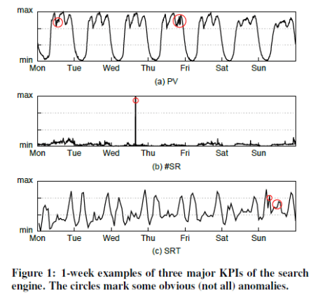
KPIs: The KPI data are the time series data with the format of (time stamp, value). In this paper, Opprentice pays attention to three kinds of KPIs: the search page view (PV), which is the number of successfully served queries; The number of slow responses of search data centers (#SR); The 80th percentile of search response time (SRT).
Anomalies: KPI time series data can also present several unexpected patterns (e.g. jitters, slow ramp ups, sudden spikes and dips) in different severity levels, such as a sudden drop by 20% or 50%.
问题和目标:
覆盖率(recall):# of true anomalous points detected / # of the anomalous points
准确率(precision):# of true anomalous points detected / # of anomalous points detected
1-FDR(false discovery rate):# of false anomalous points detected / # of anomalous points detected = 1 – precision
The quantitative goal of opprentice is precision>=0.66 and recall>=0.66.
The qualitative goal of opprentice is automatic enough so that the operators would not be involved in selecting and combining suitable detectors, or tuning them.
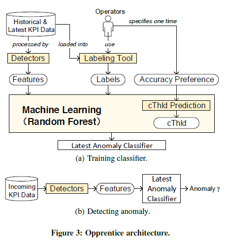
3. Opprentice Overview: (Opprentice系统的概况)
(i) Opprentice approaches the above problem through supervised machine learning.
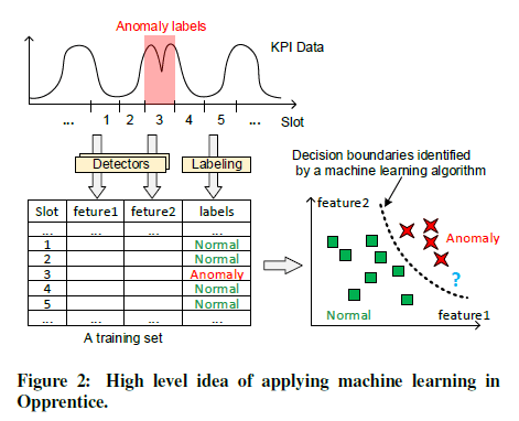
(ii) Features of the data are the results of the detectors.(Basic Detectors 来计算出特征)
(iii) The labels of the data are from operators’ experience.(人工打标签)
(iv) Addressing Challenges in Machine Learning: (机器学习遇到的挑战)
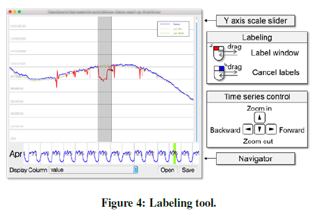
(1) Label Overhead: Opprentice has a dedicated labeling tool with a simple and convenient interaction interface. (标签的获取)
(2) Incomplete Anomaly Cases:(异常情况的不完全信息)
(3) Class Imbalance Problem: (正负样本比例不均衡)
(4) Irrelevant and Redundant Features:(无关和多余的特征)
4. Opprentice’s Design:
Architecture: Operators label the data and numerous detectors functions are feature extractors for the data.
Label Tool:
人工使用鼠标和软件进行标注工作
Detectors:
(i) Detectors As Feature Extractors: (Detector用来提取特征)
Here for each parameter detector, we sample their parameters so that we can obtain several fixed detectors, and a detector with specific sampled parameters a (detector) configuration. Thus a configuration acts as a feature extractor:
data point + configuration (detector + sample parameters) -> feature,
(ii) Choosing Detectors: (Detector的选择,目前有14种较为常见的)
Opprentice can find suitable ones from broadly selected detectors, and achieve a relatively high accuracy. Here, we implement 14 widely-used detectors in Opprentice.
Opprentice has 14 widely-used detectors:
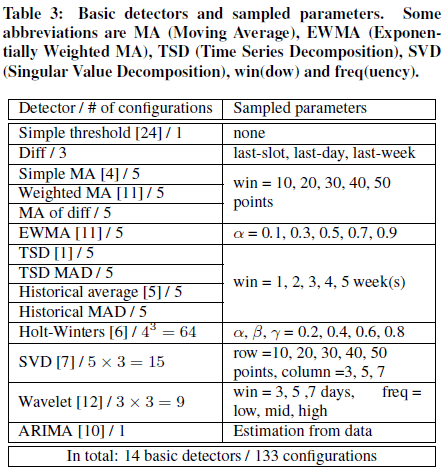
“Diff“: it simply measures anomaly severity using the differences between the current point and the point of last slot, the point of last day, and the point of last week.
“MA of diff“: it measures severity using the moving average of the difference between current point and the point of last slot.
The other 12 detectors come from previous literature. Among these detectors, there are two variants of detectors using MAD (Median Absolute Deviation) around the median, instead of the standard deviation around the mean, to measure anomaly severity.
(iii) Sampling Parameters: (Detector的参数选择方法,一种是扫描参数空间,另外一种是选择最佳的参数)
Two methods to sample the parameters of detectors.
(1) The first one is to sweep the parameter space. For example, in EWMA, we can choose  to obtain 5 typical features from EWMA; Holt-Winters has three [0,1] valued parameters
  . To choose
  , we have
  features; In ARIMA, we can estimate their “best” parameters from the data, and generate only one set of parameters, or one configuration for each detector.
Supervised Machine Learning Models:
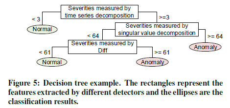
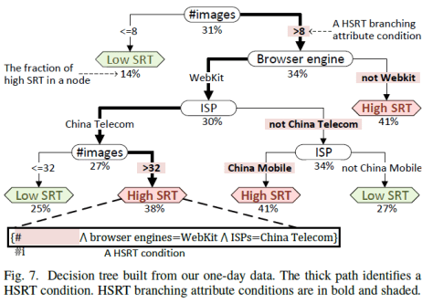
Decision Trees, logistic regression, linear support vector machines (SVMs), and naive Bayes. 下面是决策树(Decision Tree)的一个简单例子。
Random Forest is an ensemble classifier using many decision trees. It main principle is that a group of weak learners (e.g. individual decision trees) can together form a strong learner. To grow different trees, a random forest adds some elements or randomness. First, each tree is trained on subsets sampled from the original training set. Second, instead of evaluating all the features at each level, the trees only consider a random subset of the features each time. The random forest combines those trees by majority vote. The above properties of randomness and ensemble make random forest more robust to noises and perform better when faced with irrelevant and redundant features than decisions trees.
Configuring cThlds: (阈值的计算和预估)
(i) methods to select proper cThlds: offline part
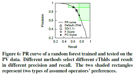
We need to figure cThlds rather than using the default one (e.g. 0.5) for two reasons.
(1) First, when faced with imbalanced data (anomalous data points are much less frequent than normal ones in data sets), machine learning algorithems typically fail to identify the anomalies (low recall) if using the default cThlds (e.g. 0.5).
(2) Second, operators have their own preference regarding the precision and recall of anomaly detection.
The metric to evaluate the precision and recall are:
(1) F-Score: F-Score = 2*precision*recall/(precision+recall).
(2) SD(1,1): it selects the point with the shortest Euclidean distance to the upper right corner where the precision and the recall are both perfect.
(3) PC-Score: (本文中采用这种评估指标来选择合适的阈值)
If r>=R and p>=P, then PC-Score(r,p)=2*r*p/(r+p) + 1; else PC-Score(r,p)=2*r*p/(r+p). Here, R and P are from the operators’ preference “recall>=R and precision>=P”. Since the F-Score is no more than 1, then we can choose the cThld corresponding to the point with the largest PC-Score.
(ii) EWMA Based cThld Prediction: (基于EWMA方法的阈值预估算法)
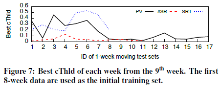
In online detection, we need to predict cThlds for detecting future data.
Use EWMA to predict the cThld of the i-th week ( or the i-th test set) based on the historical best cThlds. Specially, EWMA works as follows:
If  , then
  5-fold prediction
Else  , then
  +
+ , where
  is the best cThld of the (i-1)-th week.
  is the predicted cThld of the i-th week, and also the one used for detecting the i-th week data.
 ![\alpha\in [0,1]](https://s0.wp.com/latex.php?latex=%5Calpha%5Cin+%5B0%2C1%5D&bg=ffffff&fg=2b2b2b&s=0&c=20201002) is the smoothing constant.
is the smoothing constant.
For the first week, we use 5-fold cross-validation to initialize  . As
. As  increases, EWMA gives the recent best cThlds more influences in the prediction. We use
  in this paper.
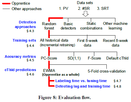
5. Evaluation(系统评估)
在 Opprentice 系统中,红色表示 Opprentice 系统的方法,黑色表示其他额外的方法。
Opprentice has 14 detectors with about 9500 lines of Python, R and C++ code. The machine learning block is based on the scikit-learn library.
Random Forest is better than decision trees, logistic regression, linear support vector machines (SVMs), and naive Bayes.


 is when a query is submitted;
  is when the result HTML file has been downloaded;
  is when a brower finishes parsing the HTML;
  is when the page is completely rendered. SRT is measured by
  , the user-received search response time.
 is the server response time of the HTML file, which is recorded by servers;
  is the network transmission time of the HTML file;
  is the browser parsing time of the HTML;
  is the remaining time spent before the page is rendered, e.g. download time of images from image servers.
 ,
, affects SRT.
 ? What SRT components (e.g.
  and
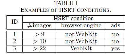
and  to get a variant condition type
  . In the past days, we have the number of HSRT events in total, the number of HSRT events in condition
  . As a result, we believe the historical data based comparison can provide a reasonable estimate of the attribute effects. The comparison between
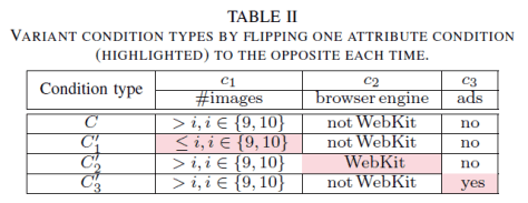
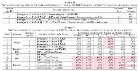
 (row 7)?
 (row 5, 10, 11, 12)?