http://www.jianshu.com/p/e112012a4b2d
cs224d-Day 6: 快速入门 Tensorflow
本文是学习这个视频课程系列的笔记,课程链接是 youtube 上的,
讲的很好,浅显易懂,入门首选, 而且在github有代码,
想看视频的也可以去他的优酷里的频道找。
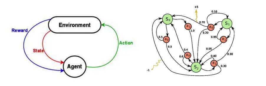
神经网络是一种数学模型,是存在于计算机的神经系统,由大量的神经元相连接并进行计算,在外界信息的基础上,改变内部的结构,常用来对输入和输出间复杂的关系进行建模。
神经网络由大量的节点和之间的联系构成,负责传递信息和加工信息,神经元也可以通过训练而被强化。
这个图就是一个神经网络系统,它由很多层构成。输入层就是负责接收信息,比如说一只猫的图片。输出层就是计算机对这个输入信息的认知,它是不是猫。隐藏层就是对输入信息的加工处理。

神经网络是如何被训练的,首先它需要很多数据。比如他要判断一张图片是不是猫。就要输入上千万张的带有标签的猫猫狗狗的图片,然后再训练上千万次。
神经网络训练的结果有对的也有错的,如果是错误的结果,将被当做非常宝贵的经验,那么是如何从经验中学习的呢?就是对比正确答案和错误答案之间的区别,然后把这个区别反向的传递回去,对每个相应的神经元进行一点点的改变。那么下一次在训练的时候就可以用已经改进一点点的神经元去得到稍微准确一点的结果。
神经网络是如何训练的呢?每个神经元都有属于它的激活函数,用这些函数给计算机一个刺激行为。

在第一次给计算机看猫的图片的时候,只有部分的神经元被激活,被激活的神经元所传递的信息是对输出结果最有价值的信息。如果输出的结果被判定为是狗,也就是说是错误的了,那么就会修改神经元,一些容易被激活的神经元会变得迟钝,另外一些神经元会变得敏感。这样一次次的训练下去,所有神经元的参数都在被改变,它们变得对真正重要的信息更为敏感。


Tensorflow 是谷歌开发的深度学习系统,用它可以很快速地入门神经网络。
它可以做分类,也可以做拟合问题,就是要把这个模式给模拟出来。

这是一个基本的神经网络的结构,有输入层,隐藏层,和输出层。
每一层点开都有它相应的内容,函数和功能。

那我们要做的就是要建立一个这样的结构,然后把数据喂进去。
把数据放进去后它就可以自己运行,TensorFlow 翻译过来就是向量在里面飞。
这个动图的解释就是,在输入层输入数据,然后数据飞到隐藏层飞到输出层,用梯度下降处理,梯度下降会对几个参数进行更新和完善,更新后的参数再次跑到隐藏层去学习,这样一直循环直到结果收敛。

今天一口气把整个系列都学完了,先来一段完整的代码,然后解释重要的知识点!
1. 搭建神经网络基本流程
定义添加神经层的函数
1.训练的数据
2.定义节点准备接收数据
3.定义神经层:隐藏层和预测层
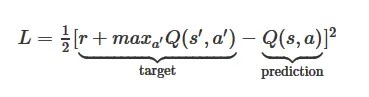
4.定义 loss 表达式
5.选择 optimizer 使 loss 达到最小
然后对所有变量进行初始化,通过 sess.run optimizer,迭代 1000 次进行学习:
import tensorflow as tf
import numpy as np

# 添加层
def add_layer(inputs, in_size, out_size, activation_function=None):
    # add one more layer and return the output of this layer
    Weights = tf.Variable(tf.random_normal([in_size, out_size]))
    biases = tf.Variable(tf.zeros([1, out_size]) + 0.1)
    Wx_plus_b = tf.matmul(inputs, Weights) + biases
    if activation_function is None:
        outputs = Wx_plus_b
    else:
        outputs = activation_function(Wx_plus_b)
    return outputs

# 1.训练的数据
# Make up some real data
x_data = np.linspace(-1,1,300)[:, np.newaxis]
noise = np.random.normal(0, 0.05, x_data.shape)
y_data = np.square(x_data) - 0.5 + noise

# 2.定义节点准备接收数据
# define placeholder for inputs to network
xs = tf.placeholder(tf.float32, [None, 1])
ys = tf.placeholder(tf.float32, [None, 1])

# 3.定义神经层:隐藏层和预测层
# add hidden layer 输入值是 xs,在隐藏层有 10 个神经元
l1 = add_layer(xs, 1, 10, activation_function=tf.nn.relu)
# add output layer 输入值是隐藏层 l1,在预测层输出 1 个结果
prediction = add_layer(l1, 10, 1, activation_function=None)

# 4.定义 loss 表达式
# the error between prediciton and real data
loss = tf.reduce_mean(tf.reduce_sum(tf.square(ys - prediction),
                     reduction_indices=[1]))

# 5.选择 optimizer 使 loss 达到最小
# 这一行定义了用什么方式去减少 loss,学习率是 0.1
train_step = tf.train.GradientDescentOptimizer(0.1).minimize(loss)


# important step 对所有变量进行初始化
init = tf.initialize_all_variables()
sess = tf.Session()
# 上面定义的都没有运算,直到 sess.run 才会开始运算
sess.run(init)

# 迭代 1000 次学习,sess.run optimizer
for i in range(1000):
    # training train_step 和 loss 都是由 placeholder 定义的运算,所以这里要用 feed 传入参数
    sess.run(train_step, feed_dict={xs: x_data, ys: y_data})
    if i % 50 == 0:
        # to see the step improvement
        print(sess.run(loss, feed_dict={xs: x_data, ys: y_data}))
2. 主要步骤的解释:
- 之前写过一篇文章 TensorFlow 入门 讲了 tensorflow 的安装,这里使用时直接导入:
import tensorflow as tf
import numpy as np- 导入或者随机定义训练的数据 x 和 y:
x_data = np.random.rand(100).astype(np.float32)
y_data = x_data*0.1 + 0.3- 先定义出参数 Weights,biases,拟合公式 y,误差公式 loss:
Weights = tf.Variable(tf.random_uniform([1], -1.0, 1.0))
biases = tf.Variable(tf.zeros([1]))
y = Weights*x_data + biases
loss = tf.reduce_mean(tf.square(y-y_data))- 选择 Gradient Descent 这个最基本的 Optimizer:
optimizer = tf.train.GradientDescentOptimizer(0.5)- 神经网络的 key idea,就是让 loss 达到最小:
train = optimizer.minimize(loss)- 前面是定义,在运行模型前先要初始化所有变量:
init = tf.initialize_all_variables()- 接下来把结构激活,sesseion像一个指针指向要处理的地方:
sess = tf.Session()- init 就被激活了,不要忘记激活:
sess.run(init)- 训练201步:
for step in range(201):- 要训练 train,也就是 optimizer:
sess.run(train)- 每 20 步打印一下结果,sess.run 指向 Weights,biases 并被输出:
if step % 20 == 0:
print(step, sess.run(Weights), sess.run(biases))
所以关键的就是 y,loss,optimizer 是如何定义的。
3. TensorFlow 基本概念及代码:
在 TensorFlow 入门 也提到了几个基本概念,这里是几个常见的用法。
- Session
矩阵乘法:tf.matmul
product = tf.matmul(matrix1, matrix2) # matrix multiply np.dot(m1, m2)定义 Session,它是个对象,注意大写:
sess = tf.Session()result 要去 sess.run 那里取结果:
result = sess.run(product)- Variable
用 tf.Variable 定义变量,与python不同的是,必须先定义它是一个变量,它才是一个变量,初始值为0,还可以给它一个名字 counter:
state = tf.Variable(0, name='counter')将 new_value 加载到 state 上,counter就被更新:
update = tf.assign(state, new_value)如果有变量就一定要做初始化:
init = tf.initialize_all_variables() # must have if define variable- placeholder:
要给节点输入数据时用 placeholder,在 TensorFlow 中用placeholder 来描述等待输入的节点,只需要指定类型即可,然后在执行节点的时候用一个字典来“喂”这些节点。相当于先把变量 hold 住,然后每次从外部传入data,注意 placeholder 和 feed_dict 是绑定用的。
这里简单提一下 feed 机制, 给 feed 提供数据,作为 run()
调用的参数, feed 只在调用它的方法内有效, 方法结束, feed 就会消失。
import tensorflow as tf

input1 = tf.placeholder(tf.float32)
input2 = tf.placeholder(tf.float32)
ouput = tf.mul(input1, input2)

with tf.Session() as sess:
  print(sess.run(ouput, feed_dict={input1: [7.], input2: [2.]}))
4. 神经网络基本概念
- 激励函数:
例如一个神经元对猫的眼睛敏感,那当它看到猫的眼睛的时候,就被激励了,相应的参数就会被调优,它的贡献就会越大。
下面是几种常见的激活函数:
x轴表示传递过来的值,y轴表示它传递出去的值:

激励函数在预测层,判断哪些值要被送到预测结果那里:

TensorFlow 常用的 activation function
- 添加神经层:
输入参数有 inputs, in_size, out_size, 和 activation_function
import tensorflow as tf

def add_layer(inputs, in_size, out_size,  activation_function=None):

  Weights = tf.Variable(tf.random_normal([in_size, out_size]))
  biases = tf.Variable(tf.zeros([1, out_size]) + 0.1)
  Wx_plus_b = tf.matmul(inputs, Weights) + biases

  if activation_function is None:
    outputs = Wx_plus_b
  else:
    outputs = activation_function(Wx_plus_b)

return outputs- 分类问题的 loss 函数 cross_entropy :
# the error between prediction and real data
# loss 函数用 cross entropy
cross_entropy = tf.reduce_mean(-tf.reduce_sum(ys * tf.log(prediction),
                                              reduction_indices=[1]))       # loss
train_step = tf.train.GradientDescentOptimizer(0.5).minimize(cross_entropy)- overfitting:
下面第三个图就是 overfitting,就是过度准确地拟合了历史数据,而对新数据预测时就会有很大误差:

Tensorflow 有一个很好的工具, 叫做dropout, 只需要给予它一个不被 drop 掉的百分比,就能很好地降低 overfitting。
dropout 是指在深度学习网络的训练过程中,按照一定的概率将一部分神经网络单元暂时从网络中丢弃,相当于从原始的网络中找到一个更瘦的网络,这篇博客中讲的非常详细

代码实现就是在 add layer 函数里加上 dropout, keep_prob 就是保持多少不被 drop,在迭代时在 sess.run 中被 feed:
def add_layer(inputs, in_size, out_size, layer_name, activation_function=None, ):
    # add one more layer and return the output of this layer
    Weights = tf.Variable(tf.random_normal([in_size, out_size]))
    biases = tf.Variable(tf.zeros([1, out_size]) + 0.1, )
    Wx_plus_b = tf.matmul(inputs, Weights) + biases

    # here to dropout
    # 在 Wx_plus_b 上drop掉一定比例
    # keep_prob 保持多少不被drop,在迭代时在 sess.run 中 feed
    Wx_plus_b = tf.nn.dropout(Wx_plus_b, keep_prob)

    if activation_function is None:
        outputs = Wx_plus_b
    else:
        outputs = activation_function(Wx_plus_b, )
    tf.histogram_summary(layer_name + '/outputs', outputs)
    return outputs
5. 可视化 Tensorboard
Tensorflow 自带 tensorboard ,可以自动显示我们所建造的神经网络流程图:

就是用 with tf.name_scope 定义各个框架,注意看代码注释中的区别:
import tensorflow as tf


def add_layer(inputs, in_size, out_size, activation_function=None):
    # add one more layer and return the output of this layer
    # 区别:大框架,定义层 layer,里面有 小部件
    with tf.name_scope('layer'):
        # 区别:小部件
        with tf.name_scope('weights'):
            Weights = tf.Variable(tf.random_normal([in_size, out_size]), name='W')
        with tf.name_scope('biases'):
            biases = tf.Variable(tf.zeros([1, out_size]) + 0.1, name='b')
        with tf.name_scope('Wx_plus_b'):
            Wx_plus_b = tf.add(tf.matmul(inputs, Weights), biases)
        if activation_function is None:
            outputs = Wx_plus_b
        else:
            outputs = activation_function(Wx_plus_b, )
        return outputs


# define placeholder for inputs to network
# 区别:大框架,里面有 inputs x,y
with tf.name_scope('inputs'):
    xs = tf.placeholder(tf.float32, [None, 1], name='x_input')
    ys = tf.placeholder(tf.float32, [None, 1], name='y_input')

# add hidden layer
l1 = add_layer(xs, 1, 10, activation_function=tf.nn.relu)
# add output layer
prediction = add_layer(l1, 10, 1, activation_function=None)

# the error between prediciton and real data
# 区别:定义框架 loss
with tf.name_scope('loss'):
    loss = tf.reduce_mean(tf.reduce_sum(tf.square(ys - prediction),
                                        reduction_indices=[1]))

# 区别:定义框架 train
with tf.name_scope('train'):
    train_step = tf.train.GradientDescentOptimizer(0.1).minimize(loss)

sess = tf.Session()

# 区别:sess.graph 把所有框架加载到一个文件中放到文件夹"logs/"里
# 接着打开terminal,进入你存放的文件夹地址上一层,运行命令 tensorboard --logdir='logs/'
# 会返回一个地址,然后用浏览器打开这个地址,在 graph 标签栏下打开
writer = tf.train.SummaryWriter("logs/", sess.graph)
# important step
sess.run(tf.initialize_all_variables())
运行完上面代码后,打开 terminal,进入你存放的文件夹地址上一层,运行命令 tensorboard –logdir=’logs/’ 后会返回一个地址,然后用浏览器打开这个地址,点击 graph 标签栏下就可以看到流程图了:

6. 保存和加载
训练好了一个神经网络后,可以保存起来下次使用时再次加载:
import tensorflow as tf
import numpy as np

## Save to file
# remember to define the same dtype and shape when restore
W = tf.Variable([[1,2,3],[3,4,5]], dtype=tf.float32, name='weights')
b = tf.Variable([[1,2,3]], dtype=tf.float32, name='biases')

init= tf.initialize_all_variables()

saver = tf.train.Saver()

# 用 saver 将所有的 variable 保存到定义的路径
with tf.Session() as sess:
   sess.run(init)
   save_path = saver.save(sess, "my_net/save_net.ckpt")
   print("Save to path: ", save_path)


################################################

# restore variables
# redefine the same shape and same type for your variables
W = tf.Variable(np.arange(6).reshape((2, 3)), dtype=tf.float32, name="weights")
b = tf.Variable(np.arange(3).reshape((1, 3)), dtype=tf.float32, name="biases")

# not need init step

saver = tf.train.Saver()
# 用 saver 从路径中将 save_net.ckpt 保存的 W 和 b restore 进来
with tf.Session() as sess:
    saver.restore(sess, "my_net/save_net.ckpt")
    print("weights:", sess.run(W))
    print("biases:", sess.run(b))
tensorflow 现在只能保存 variables,还不能保存整个神经网络的框架,所以再使用的时候,需要重新定义框架,然后把 variables 放进去学习。
原文链接:http://www.jianshu.com/p/e112012a4b2d
著作权归作者所有,转载请联系作者获得授权,并标注“简书作者”。