
我们用科普的角度来聊聊“一维动力系统”(One-Dimensional Dynamics)。
想象一下,你有一个非常简单的规则,这个规则告诉你:根据一个点当前的位置,如何确定它下一刻的位置。然后你不断地、一遍又一遍地应用这个规则。研究这个点在“时间”(可以理解为迭代次数)推进下如何运动、最终会去哪里、系统整体会表现出什么性质的学问,就是动力系统理论。
当这个点只能在一条线上移动时(比如一条无限长的数轴,或者一个首尾相接的圆圈),我们研究的系统就叫做一维动力系统。
为什么研究“一维”?
- 简单但深刻: 一维是维度最低的情况,规则相对简单,更容易分析和理解。但别小看它,即使是最简单的一维规则,也能产生极其复杂和令人惊讶的行为(比如混沌)。
- 基础性: 理解了一维系统的行为,是理解更高维(二维、三维甚至无穷维)更复杂系统的基础。很多高维系统中的核心思想和现象(如混沌、分形、吸引子)都能在一维模型中找到原型或被深刻理解。
- 应用广泛: 虽然模型简单,但一维动力系统可以用来描述很多实际现象的简化模型,比如:
(1)种群增长: 今年昆虫的数量决定了明年的大致数量(考虑环境承载力的限制)。
(2)简单物理过程: 单摆的近似运动(在小角度时)。
(3)经济模型: 简单的市场供需关系演化。
(4)信号处理: 某些反馈机制。

一维动力系统的核心要素:
- “舞台”: 点运动的空间。主要分两类:
- 区间: 比如一条线段
[0, 1]。点不能跑出这个范围。 - 圆周: 像一个环
S¹。点跑出“右边界”会从“左边界”回来(反之亦然)。想象一个圆盘边缘的点。
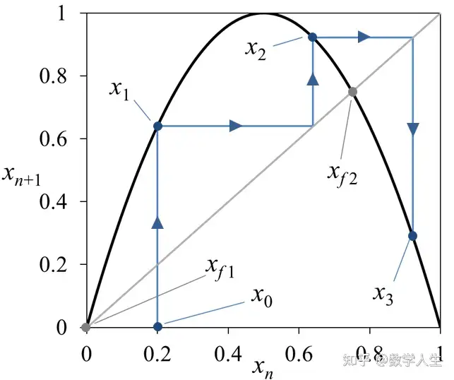
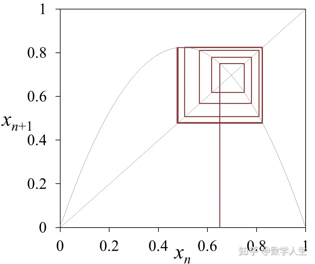
2. “规则”: 一个函数 f(x)。它定义了如何根据当前点 x 的位置,计算出下一个点 x_{n+1} = f(x_n)。这个函数通常是连续的,有时甚至是光滑的(可导的)。
3. “演员”: 一个初始点 x₀。
4. “剧情”: 点运动的轨迹 x₀, x₁ = f(x₀), x₂ = f(x₁) = f(f(x₀)), x₃ = f(f(f(x₀))), ...。这个序列 {x₀, x₁, x₂, ...} 称为轨道。
研究什么?关键问题:
- 不动点: 有没有点
x*满足f(x*) = x*?这个点就像“黑洞”,一旦到达就永远停在那里。它是系统最简单的稳定状态。 - 周期点: 有没有点
x_p满足f(f(...f(x_p)...)) = x_p(应用k次后回到自身)?这样的点会产生一个循环往复的轨道(x_p, f(x_p), f²(x_p), ..., f^{k-1}(x_p), x_p, ...),称为周期k轨道。这代表了系统的周期性行为。 - 吸引子: 大多数初始点的轨道最终会趋向于什么样的状态?是一个不动点?一个周期轨道?还是一个更复杂的、永不重复但被限制在某个区域的集合(混沌吸引子)?吸引子代表了系统长期行为的模式。
- 对初始条件的敏感性(蝴蝶效应): 这是混沌的核心特征。两个非常非常接近的初始点
x₀和y₀,经过多次迭代后,它们的轨道{x_n}和{y_n}会分道扬镳,变得毫无关系吗?如果系统具有这种性质,那么长期预测就变得极其困难。 - 拓扑共轭: 两个看起来不同的规则
f(x)和g(x),是否本质上描述了相同的动力学行为?就像一个故事用中文和英文讲述,情节一样,只是语言不同。找到这种“等价关系”有助于对系统分类。 - 分岔: 当规则
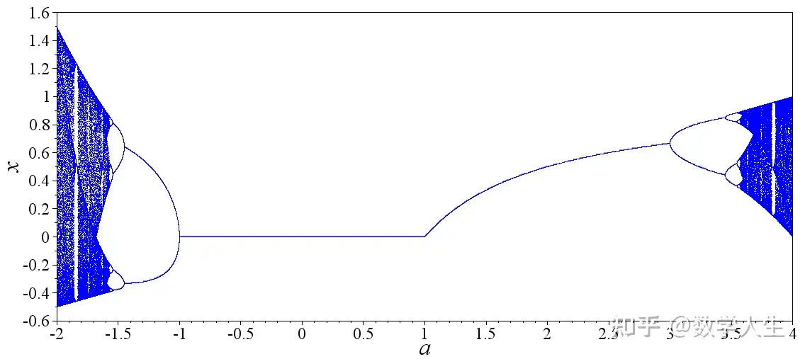
f(x)依赖于某个参数a(比如f_a(x) = a * x * (1 - x))时,随着a的变化,系统的长期行为(吸引子的类型、数量、稳定性)会发生突然的、戏剧性的变化。这就像调节一个旋钮,系统性质突然“跃变”了。
一个著名的例子:Logistic Map(逻辑斯蒂映射)
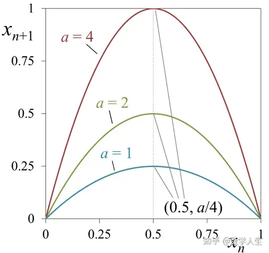
规则极其简单:f(x) = r * x * (1 - x)。其中 x 在 [0, 1] 区间内(比如可以代表种群数量占环境最大承载量的比例),r 是一个参数(比如代表繁殖率)。
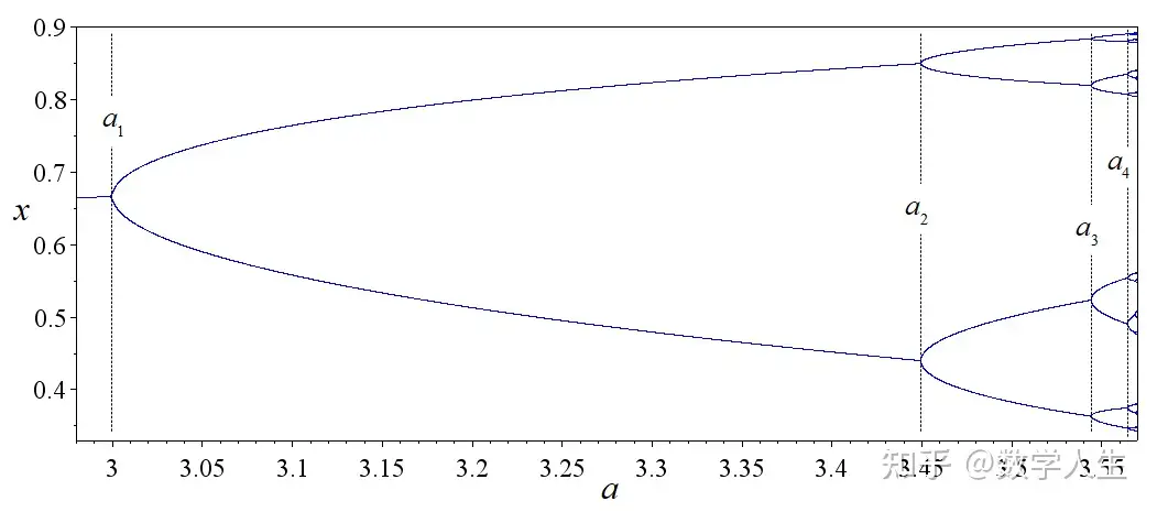
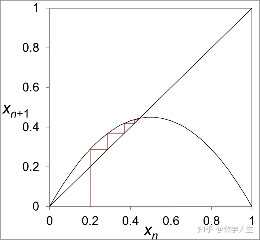
- 当
r比较小(比如r=2)时:几乎所有初始点的轨道都趋向于一个稳定的不动点。种群数量最终稳定在一个固定值。 - 当
r增大一些(比如r=3.2)时:不动点失稳,出现一个稳定的周期2轨道。种群数量开始呈现“大小年”交替振荡。 - 当
r继续增大(比如r=3.5)时:周期2失稳,出现稳定的周期4轨道。振荡模式变得更复杂。 - 当
r增大到某个临界值(约r≈3.57)以上:系统进入混沌区!轨道看起来是随机的(虽然由完全确定的规则产生),永不重复,对初始条件极其敏感。种群数量变化变得不可长期预测。在这个区域里,还能发现一些“窗口”,其中又会出现稳定的周期轨道(比如周期3)。 - 当
r=4时:混沌行为充满整个区间[0, 1],并且轨道点会稠密地分布在整个区间。
这个简单的二次函数,仅仅通过改变一个参数 r,就展现了从稳定、周期振荡到混沌的几乎所有一维动力系统的典型行为!它是一维动力系统研究的“明星模型”。
一维动力系统研究的是点在一条线(直线段或圆圈)上,按照一个确定的规则 f(x) 一步步移动的长期行为。它关注点最终会去哪里(吸引子)、是否会周期性重复、是否对起点极其敏感(混沌),以及当规则参数变化时行为如何突变(分岔)。虽然空间结构简单,但它能产生极其丰富和复杂的动力学现象,是理解更复杂系统的基础,并且在简化模型中描述了许多自然和社会现象。Logistic Map 是展示一维动力系统魅力最经典的例子。


 ;
; ;
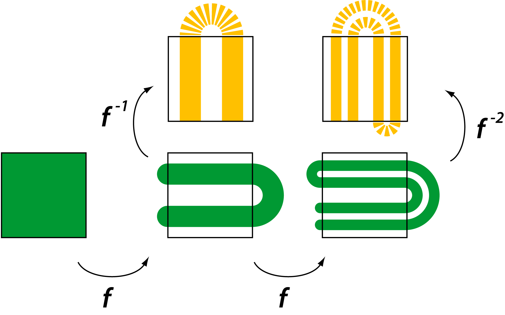
; ,如图所示。
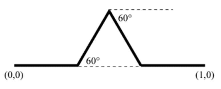
 表示向前,
表示向前, 表示左转
表示左转  表示右转
表示右转  。也就是说,每一次的迭代,都会使得总的长度变成原来的
  倍。由于
倍。由于 ,
, 个大小一致且互不重叠的小物体组成,这些小物体的形状和这个物体本身相同。若这些小物体和大物体的大小比例为
  ,也就是说小物体放大
  倍之后与大物体完全重合,那么这个几何物体的 Hausdorff 维度(豪斯多夫维数)就定义为
  ,
, 。
。 的线段可以被分成
  段(
段( ),每段的长度与原来线段的大小比例是
  (
( ),因此 Hausdorff 维度是
  。
。 个边长是
个边长是  的小正方形,每一个小正方形与原来正方形的大小比例是
  。
。 个边长是
个边长是  。
。 。
。 。
。
 。
。
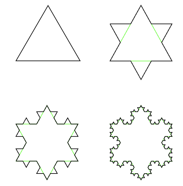
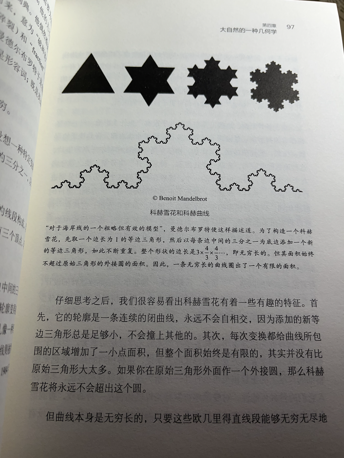
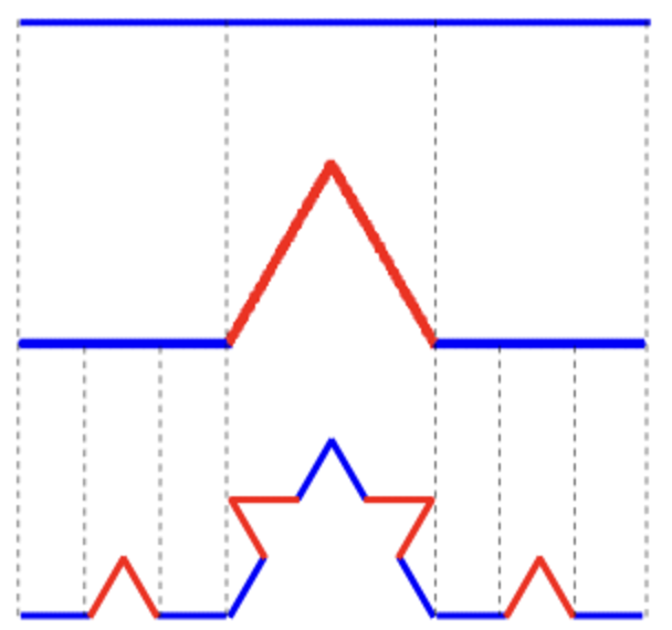
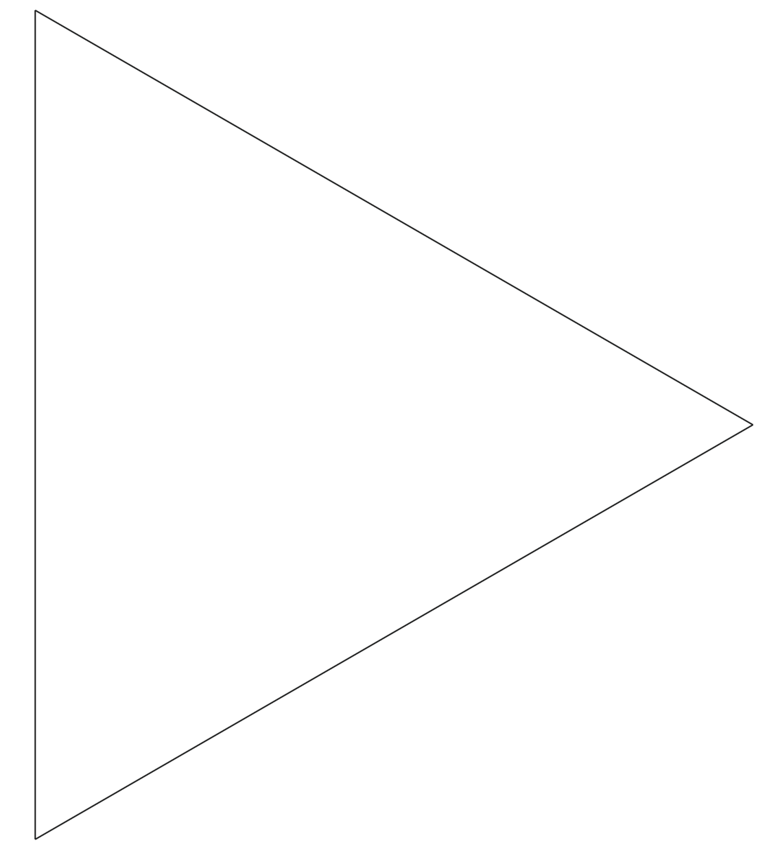
 是初始三角形的面积,
 表示第 $n$ 次迭代的三角形面积,其中
  。
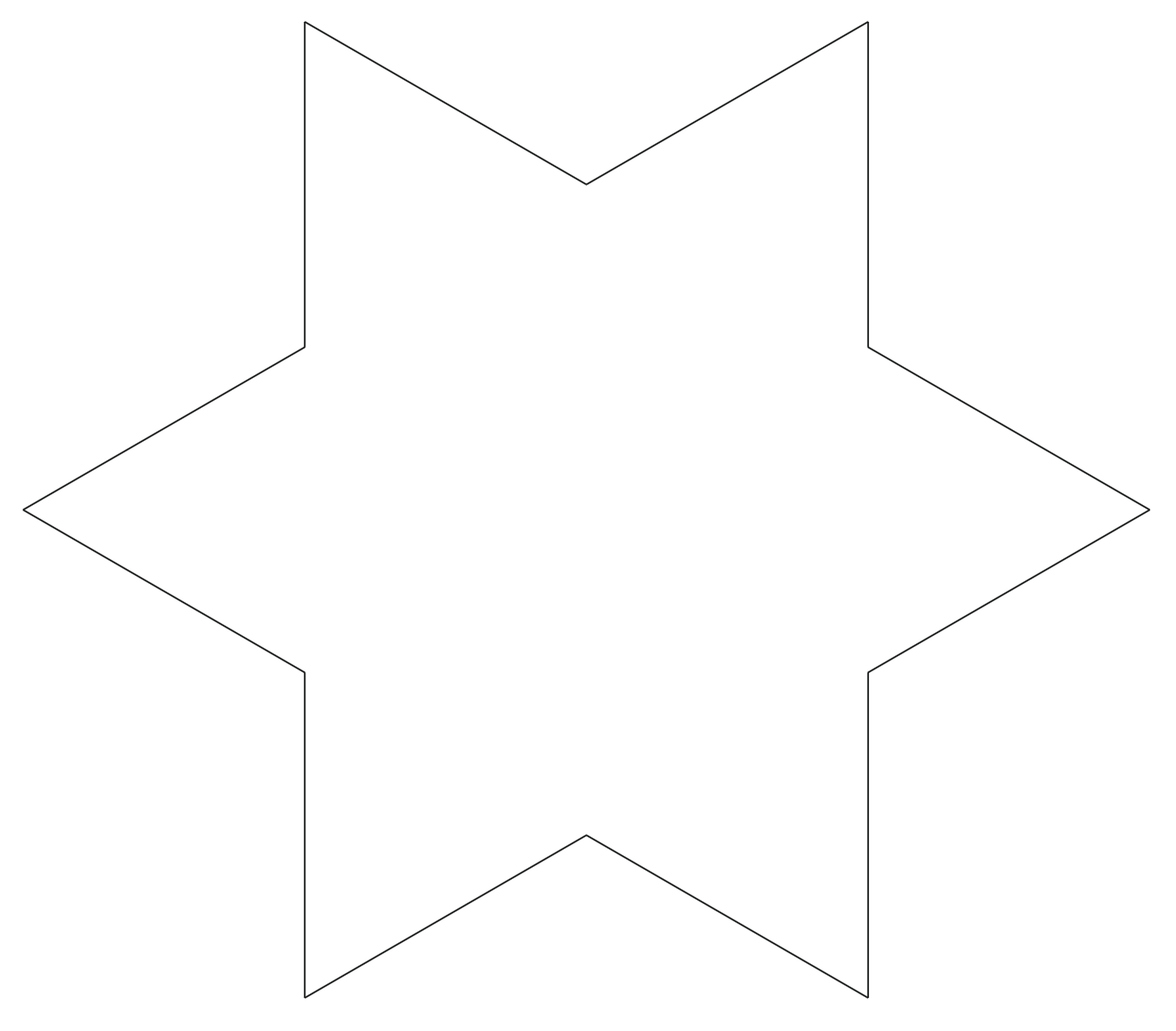
。 条,在第一次迭代的时候会生成三个小三角形,每一个小三角形的面积是初始的
  ,同时从
,同时从  条边。也就是说:
 。
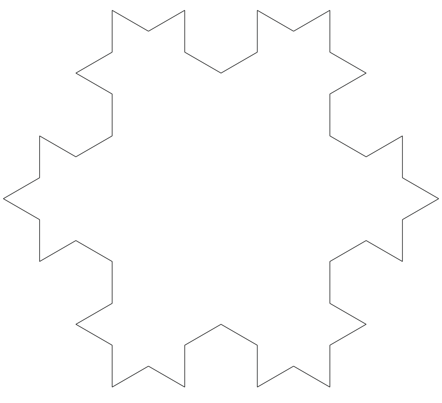
。 ,同时从
,同时从  条边。也就是说:
 。
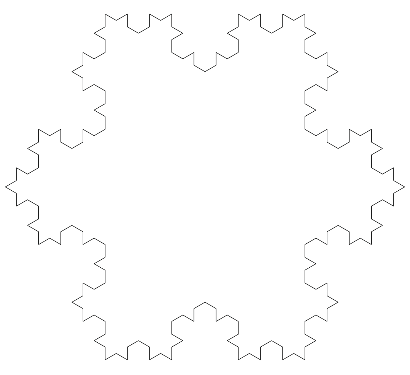
。

 。
。


 ,考察其定义域的点
  的
的  ,进一步可以研究
  的极限。
的极限。 (
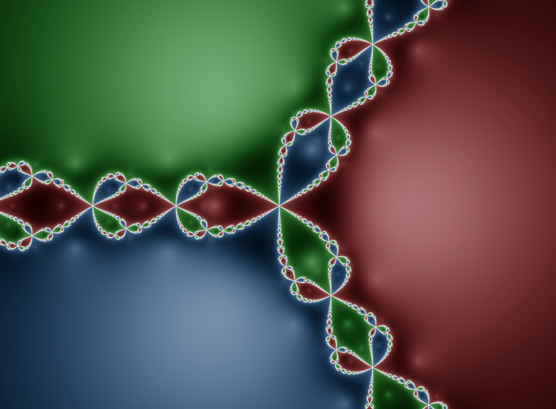
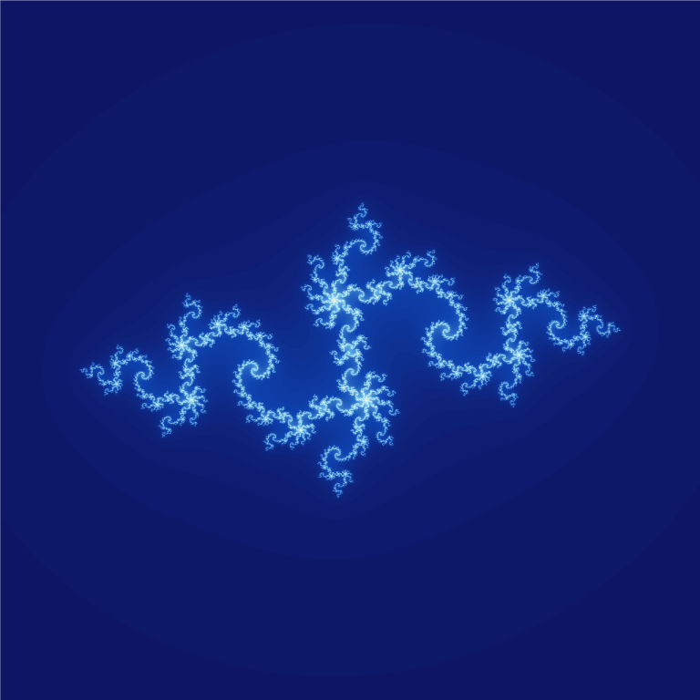
(![a\in[0,2\pi]](https://s0.wp.com/latex.php?latex=a%5Cin%5B0%2C2%5Cpi%5D&bg=ffffff&fg=2b2b2b&s=0&c=20201002) )的 Julia 集合的动图如下:
)的 Julia 集合的动图如下:


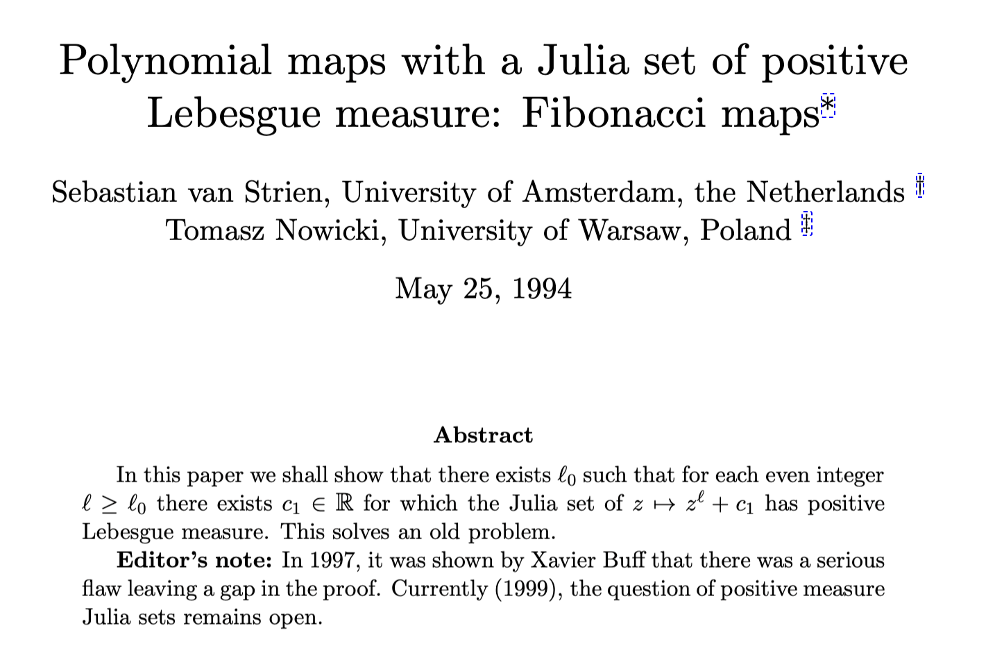
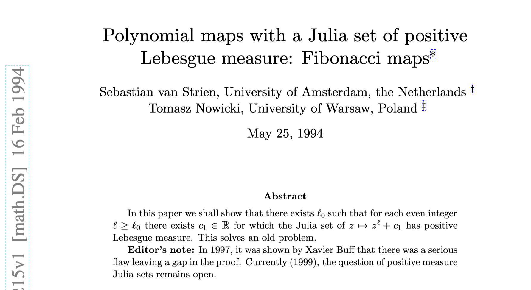
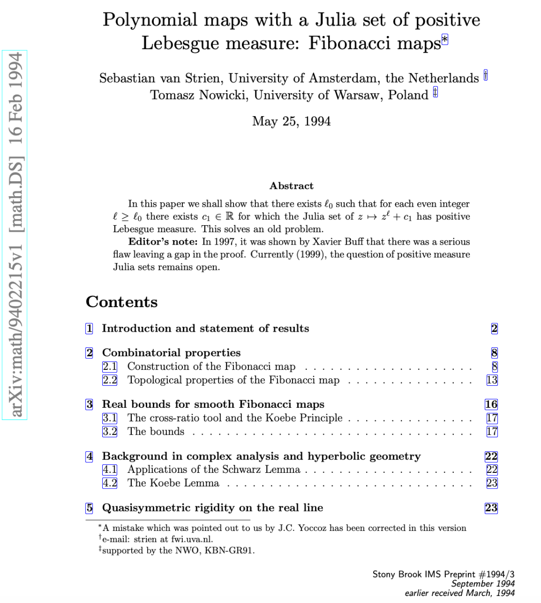
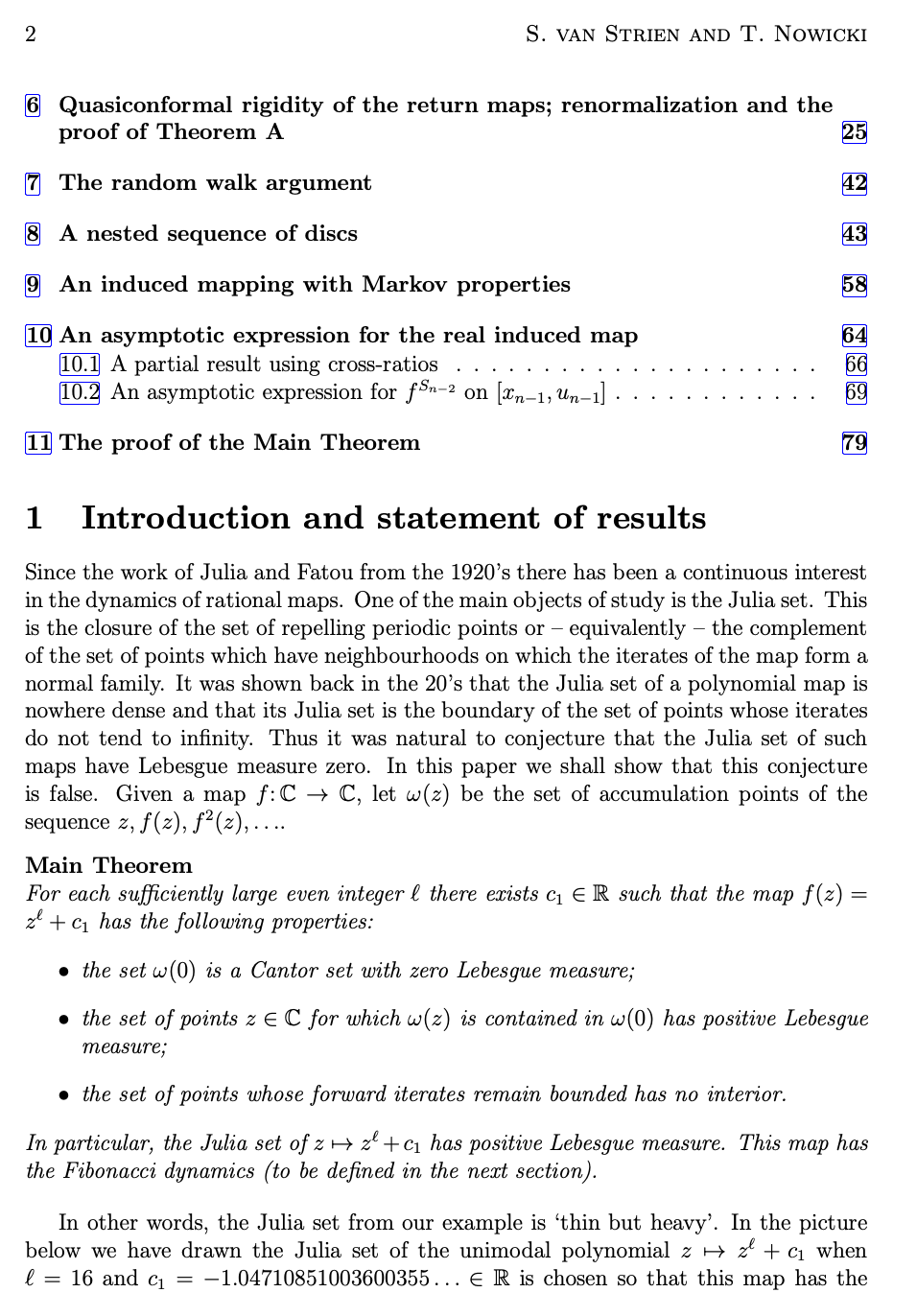
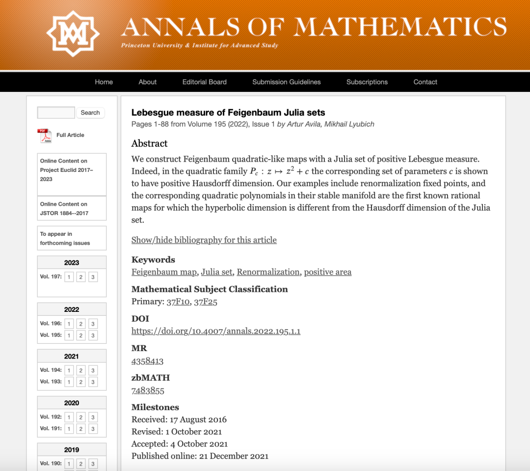
 的偶数和复数
  使得
使得  的 Julia 集合
  是正测度?
是正测度?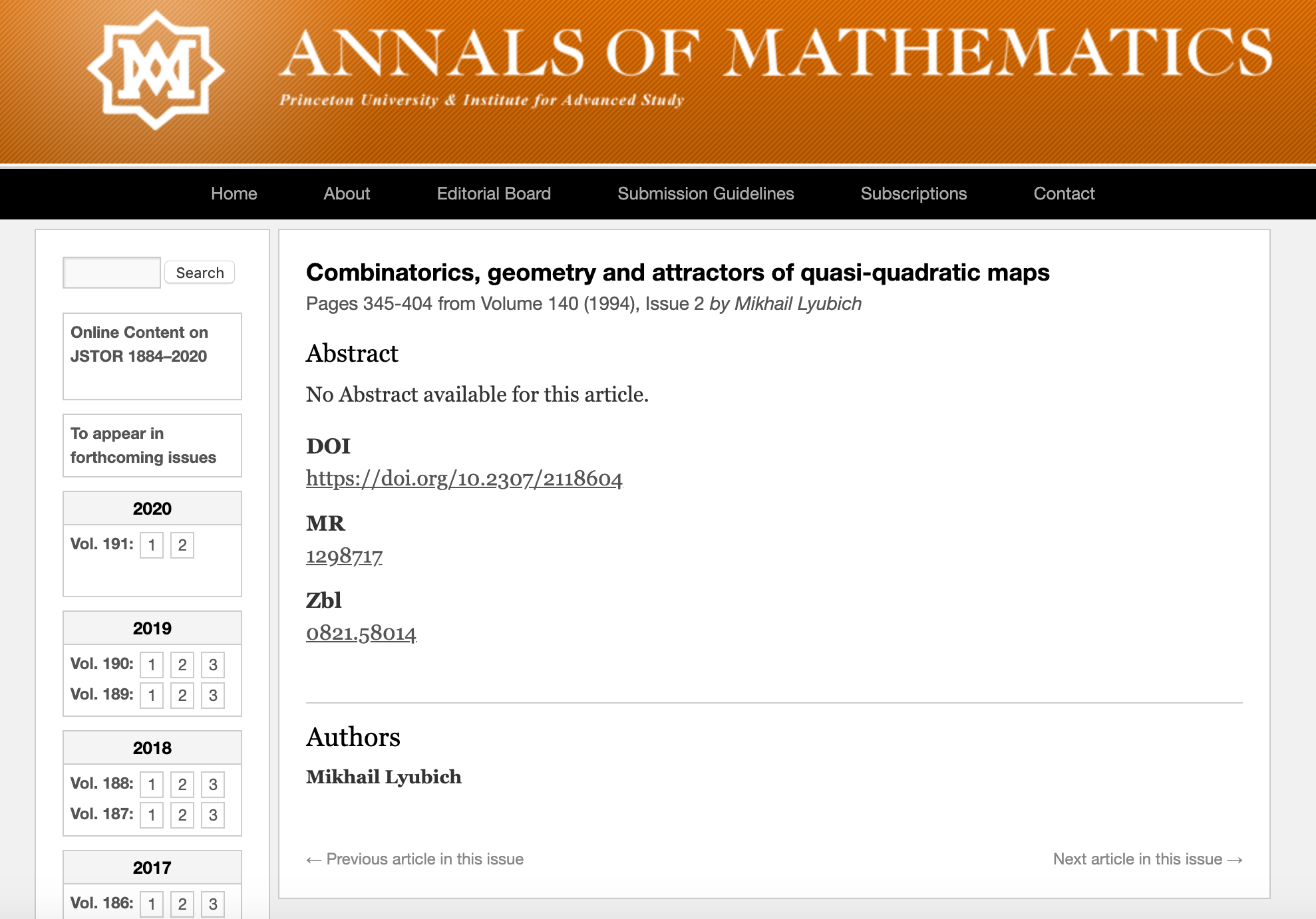

 = \sum\limits_{n=0}^{\infty} \lambda^n \cos(2\pi b^n x)")
 .
. = \sum\limits_{n=0}^{\infty} \lambda^n \phi(b^n x)")
 is a
is a  -periodic
  -function.
 because they are concrete examples of continuous but nowhere differentiable functions.
 tends to be a “fractal object” because
  = \phi(x) + \lambda f^{\phi}_{\lambda,b}(bx)")
 -function for all
  . In fact, for all
 ![{x,y\in[0,1]}](https://s0.wp.com/latex.php?latex=%7Bx%2Cy%5Cin%5B0%2C1%5D%7D&bg=ffffff&fg=000000&s=0 "{x,y\in[0,1]}") , we have
, we have - f^{\phi}_{\lambda,b}(y)}{|x-y|^{\alpha}} = \sum\limits_{n=0}^{\infty} \lambda^n b^{n\alpha} \left(\frac{\phi(b^n x) - \phi(b^n y)}{|b^n x - b^n y|^{\alpha}}\right),")
 - f^{\phi}_{\lambda,b}(y)}{|x-y|^{\alpha}} \leq \|\phi\|_{C^{\alpha}} \sum\limits_{n=0}^{\infty}(\lambda b^{\alpha})^n:=C(\phi,\alpha,\lambda,b) < \infty")
 , i.e.,
  .
.![{f:[0,1]\rightarrow\mathbb{R}}](https://s0.wp.com/latex.php?latex=%7Bf%3A%5B0%2C1%5D%5Crightarrow%5Cmathbb%7BR%7D%7D&bg=ffffff&fg=000000&s=0 "{f:[0,1]\rightarrow\mathbb{R}}") is
is)\leq 2 - \alpha")
 , the Hölder continuity condition
-f(y)|\leq C|x-y|^{\alpha}")
}") by the family
by the family _{j=1}^n}") of rectangles given by
of rectangles given by![\displaystyle R_{j,n}:=\left[\frac{j-1}{n}, \frac{j}{n}\right] \times \left[f(j/n)-\frac{C}{n^{\alpha}}, f(j/n)+\frac{C}{n^{\alpha}}\right]](https://s0.wp.com/latex.php?latex=%5Cdisplaystyle+R_%7Bj%2Cn%7D%3A%3D%5Cleft%5B%5Cfrac%7Bj-1%7D%7Bn%7D%2C+%5Cfrac%7Bj%7D%7Bn%7D%5Cright%5D+%5Ctimes+%5Cleft%5Bf%28j%2Fn%29-%5Cfrac%7BC%7D%7Bn%5E%7B%5Calpha%7D%7D%2C+f%28j%2Fn%29%2B%5Cfrac%7BC%7D%7Bn%5E%7B%5Calpha%7D%7D%5Cright%5D&bg=ffffff&fg=000000&s=0 "\displaystyle R_{j,n}:=\left[\frac{j-1}{n}, \frac{j}{n}\right] \times \left[f(j/n)-\frac{C}{n^{\alpha}}, f(j/n)+\frac{C}{n^{\alpha}}\right]")
}") . In fact, since
. In fact, since \leq 4C/n^{\alpha}}") for each
for each  , we have
^d\leq n\left(\frac{4C}{n^{\alpha}}\right)^d = (4C)^{1/\alpha} < \infty")
 . Because
 \leq 1/\alpha}") . Of course, this bound is certainly suboptimal for
. Of course, this bound is certainly suboptimal for  (because we know that
 \leq 2 < 1/\alpha}") anyway).Fortunately, we can refine the covering
anyway).Fortunately, we can refine the covering }") by taking into account that each rectangle
by taking into account that each rectangle  tends to be more vertical than horizontal (i.e., its height
  is usually larger than its width
  ). More precisely, we can divide each rectangle
  squares, say
 has diameter
  . In this way, we obtain a covering
 }") of
of  such that
^d \leq n\cdot n^{1-\alpha}\cdot\left(\frac{2}{n}\right)^d\leq (2C)^{2-\alpha}<\infty")
 . Since
 \leq 2-\alpha")
) = 2 + \frac{\log\lambda}{\log b} < 2")
) \geq 2 + \frac{\log\lambda}{\log b}")
 integer and for all
 ) = 2 + \frac{\log\lambda}{\log b}")
 a
a >1}") such that
such that) = 2 + \frac{\log\lambda}{\log b}")
 .
. such that
 .
. and
and  is large.
 = f^{\phi}_{\lambda,b}(x)}") for all
for all  . In particular, if
 }") is an invariant repeller for the endomorphism
is an invariant repeller for the endomorphism  given by
 = \left(bx\textrm{ mod }1, \frac{y-\phi(x)}{\lambda}\right)")
}") led Ledrappier to the following criterion for the validity of Mandelbrot’s conjecture when
led Ledrappier to the following criterion for the validity of Mandelbrot’s conjecture when  the alphabet
  . The unstable manifolds of
  through
 )")
 ,
,  , and
, and:=\sum\limits_{n=0}^{\infty} \gamma^n \phi'\left(\frac{x + u_1 + u_2 b + \dots + u_n b^{n-1}}{b^n}\right)")
)_*\mathbb{P}}") of the Bernoulli measure
of the Bernoulli measure  on
on  (induced by the discrete measure assigning weight
  to each letter of the alphabet
  of the expanding endomorphism
  ,
, = (bx\textrm{ mod }1, \gamma y + \psi(x)),")
 and
and =\phi'(x)}") . In plain terms, this means that
. In plain terms, this means that \ \ \ \ \ (1)")
 -invariant probability measure which is absolutely continuous along unstable manifolds (see
  have important consequences for the fractal geometry of the graph
 =1}") , i.e.,
, i.e.,)}{\log r} = 1 \textrm{ for } m_x\textrm{-a.e. } z")
}") has Hausdorff dimension
has Hausdorff dimension = 2 + \frac{\log\lambda}{\log b}")
\geq 2 + \frac{\log\lambda}{\log b}}") . By
. By  supported on
  := \textrm{ ess }\inf \underline{d}(\nu,x) \geq 2 + \frac{\log\lambda}{\log b}")
:=\liminf\limits_{r\rightarrow 0}\log \nu(B(x,r))/\log r}") . Finally, the main point is that the assumptions in Ledrappier theorem allow to prove that the measure
. Finally, the main point is that the assumptions in Ledrappier theorem allow to prove that the measure  given by the lift to
 ![{[0,1]}](https://s0.wp.com/latex.php?latex=%7B%5B0%2C1%5D%7D&bg=ffffff&fg=000000&s=0 "{[0,1]}") via the map
via the map )}") satisfies
satisfies \geq 2 + \frac{\log\lambda}{\log b}")
 , then
 for Lebesgue almost every
  for almost every
  implies that
 ,
,  and
and  , we say that two infinite words
  are
are }") -transverse at
-transverse at  if either
-s(x_0,v)|>\varepsilon")
-s'(x_0,v)|>\delta")
 ,
,  are
are  ,
,  are
are  ; otherwise, we say that
  and
and  are
are:= \{(k,l)\in\mathcal{A}^q\times\mathcal{A}^q: (k,l) \textrm{ is } (\varepsilon,\delta)\textrm{-tangent at } x_0\}}")
:=\bigcap\limits_{\varepsilon>0}\bigcap\limits_{\delta>0} E(q,x_0;\varepsilon,\delta)}") ;
;:=\max\limits_{k\in\mathcal{A}^q}\#\{l\in\mathcal{A}^q: (k,l)\in E(q,x_0)\}}")
:=\max\limits_{x_0\in\mathbb{R}/\mathbb{Z}} e(q,x_0)}") .
. integer such that
 <(\gamma b)^q}") , then
, then
 are mutually transverse, so that they almost fill a small neighborhood
  of some point
 and
and  , one has
 =1}") . Indeed, once we know that
. Indeed, once we know that  , they can apply Tsujii’s theorem and Ledrappier’s theorem (or rather Corollary
  = \cos(2\pi x)}") . If
. If  and
and <\gamma b")
 = 2+\frac{\log\lambda}{\log b}")
 ) requires the introduction of a modified version of Tsujii’s transversality condition: roughly speaking, Shen defines a function
 \leq e(q)}") (inspired from
(inspired from <(\gamma b)^q}") for some integer
for some integer  ;
; .
.:=-2\pi\sum\limits_{n=0}^{\infty} \gamma^n \sin\left(2\pi\frac{x + u_1 + u_2 b + \dots + u_n b^{n-1}}{b^n}\right)")
=-4\pi^2\sum\limits_{n=0}^{\infty} \left(\frac{\gamma}{b}\right)^n \cos\left(2\pi\frac{x + u_1 + u_2 b + \dots + u_n b^{n-1}}{b^n}\right)")
 , the series defining
 }") converges faster than the series defining
converges faster than the series defining }") .
.\in E(1,x_0)}") , then
, then - \sin\left(2\pi\frac{x_0+l}{b}\right)\right| \leq\frac{2\gamma}{1-\gamma} \ \ \ \ \ (2)")
 - \cos\left(2\pi\frac{x_0+l}{b}\right)\right| \leq \frac{2\gamma}{b-\gamma} \ \ \ \ \ (3)")
}") as follows. Take
as follows. Take =e(1,x_0)}") , and let
, and let  be such that
 ,\dots,(k,l_{e(1)})\in E(1,x_0)}") distinct elements listed in such a way that
distinct elements listed in such a way that\leq \sin(2\pi x_{i+1})")
-1}") , where
, where /b}") .
. - \cos\left(2\pi x_{i+1}\right)\right| \leq \frac{4\gamma}{b-\gamma}")
-\cos(2\pi x_{i+1}))^2 + (\sin(2\pi x_i)-\sin(2\pi x_{i+1}))^2 = 4\sin^2(\pi(x_i-x_{i+1}))\geq 4\sin^2(\pi/b),")
-\sin(2\pi x_{i+1})|\geq \sqrt{4\sin^2\left(\frac{\pi}{b}\right) - \left(\frac{4\gamma}{b-\gamma}\right)^2} \ \ \ \ \ (4)")
 - \left(\frac{4\gamma}{b-\gamma}\right)^2} > \frac{4}{b} \ \ \ \ \ (5)")
}") if
if }") ;
; ;
;}{\frac{4\gamma}{b-\gamma}}\rightarrow \frac{2\pi}{4\gamma} (< \frac{5}{3})}") as
as  , and
, and  - \frac{4\gamma}{b-\gamma} \rightarrow (2\pi-4\gamma)\frac{1}{b} (>\frac{2}{b})}") as
as  ).
).-\sin(2\pi x_{i+1})| > 4/b")
-1}") .
.\leq\sin(2\pi x_2)\leq\dots\leq\sin(2\pi x_{e(1)})\leq 1}") , the previous estimate implies that
, the previous estimate implies that-1)<\sum\limits_{i=1}^{e(1)-1}(\sin(2\pi x_{i+1}) - \sin(2\pi x_i)) = \sin(2\pi x_{e(1)}) - \sin(2\pi x_1)\leq 2,")
<1+\frac{b}{2}")
 ,
, <1+\frac{b}{2}<\gamma b")
 , we say that an interval
  is symmetric if
  where
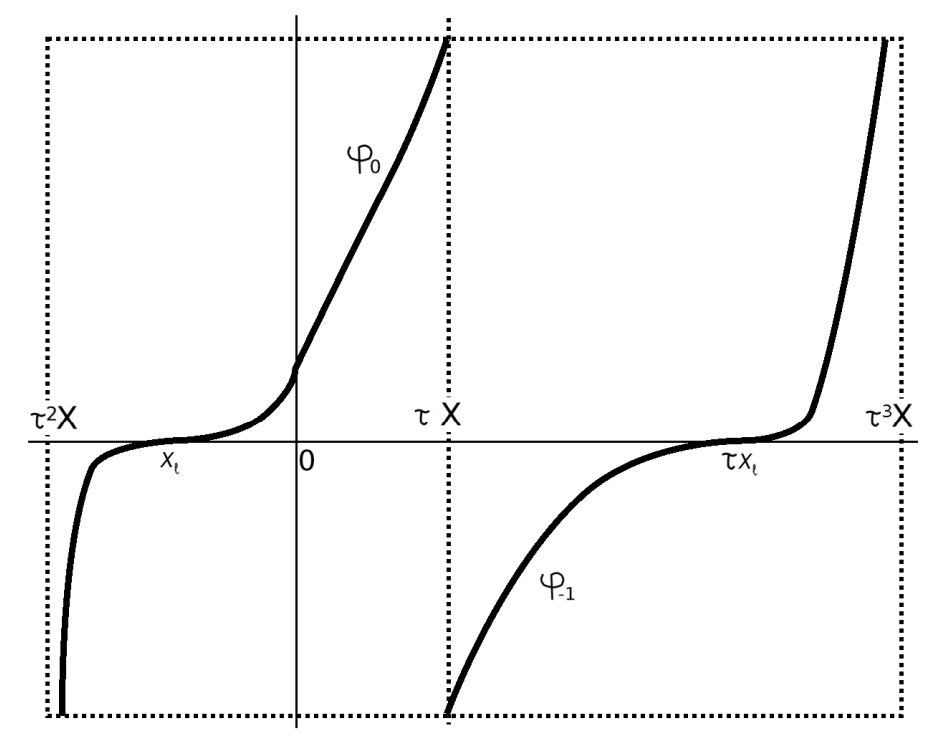
where ![\tau:[-1,1]\rightarrow [-1,1]](https://s0.wp.com/latex.php?latex=%5Ctau%3A%5B-1%2C1%5D%5Crightarrow+%5B-1%2C1%5D&bg=ffffff&fg=2b2b2b&s=0&c=20201002) is so that
is so that  and
and  if
if  . Furthermore, for each symmetric interval
 let
let  be the minimal positive integer with
  and let
 the Poincare map or transfer map to
  to
to ![f:[-1,1]\rightarrow [-1,1]](https://s0.wp.com/latex.php?latex=f%3A%5B-1%2C1%5D%5Crightarrow+%5B-1%2C1%5D&bg=ffffff&fg=2b2b2b&s=0&c=20201002) be a unimodal map with one non-flat critical point with negative Schwarzian derivative and without attracting periodic points. Then there exists
be a unimodal map with one non-flat critical point with negative Schwarzian derivative and without attracting periodic points. Then there exists  and a sequence os symmetric intervals
  around the turning point which shrink to
  such that
  contains a
  scaled neighbourhood of
  and such that the following properties hold.
 is constant.
 be a component of the domain
  such that
  is monotone,
  and
and  . Here
  is the transfer time on
  .
. such that
 to
to  .
. can be written as
  where the distortion of
  is universally bounded by
  (Here
(Here  ) has either zero or full Lebesgue measure. An alternative way to define this notation of ergodicity goes as follows:
  such that
  has Lebesgue measure zero, at most one of these sets has positive Lebesgue measure. (Here
  .)
.) ,
,  for almost all
  (in which case it is called a solenoidal attractor);
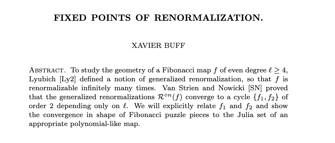
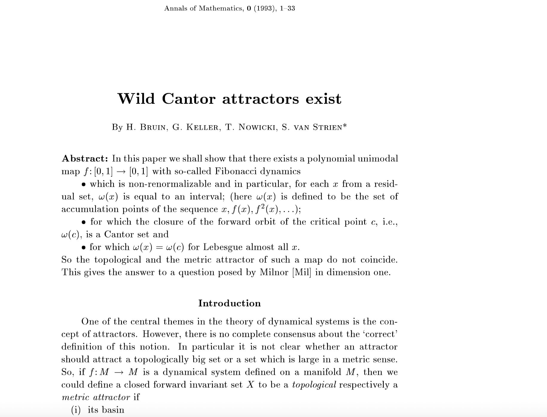
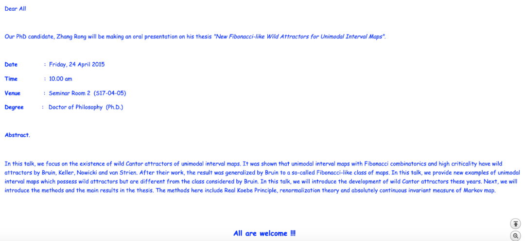
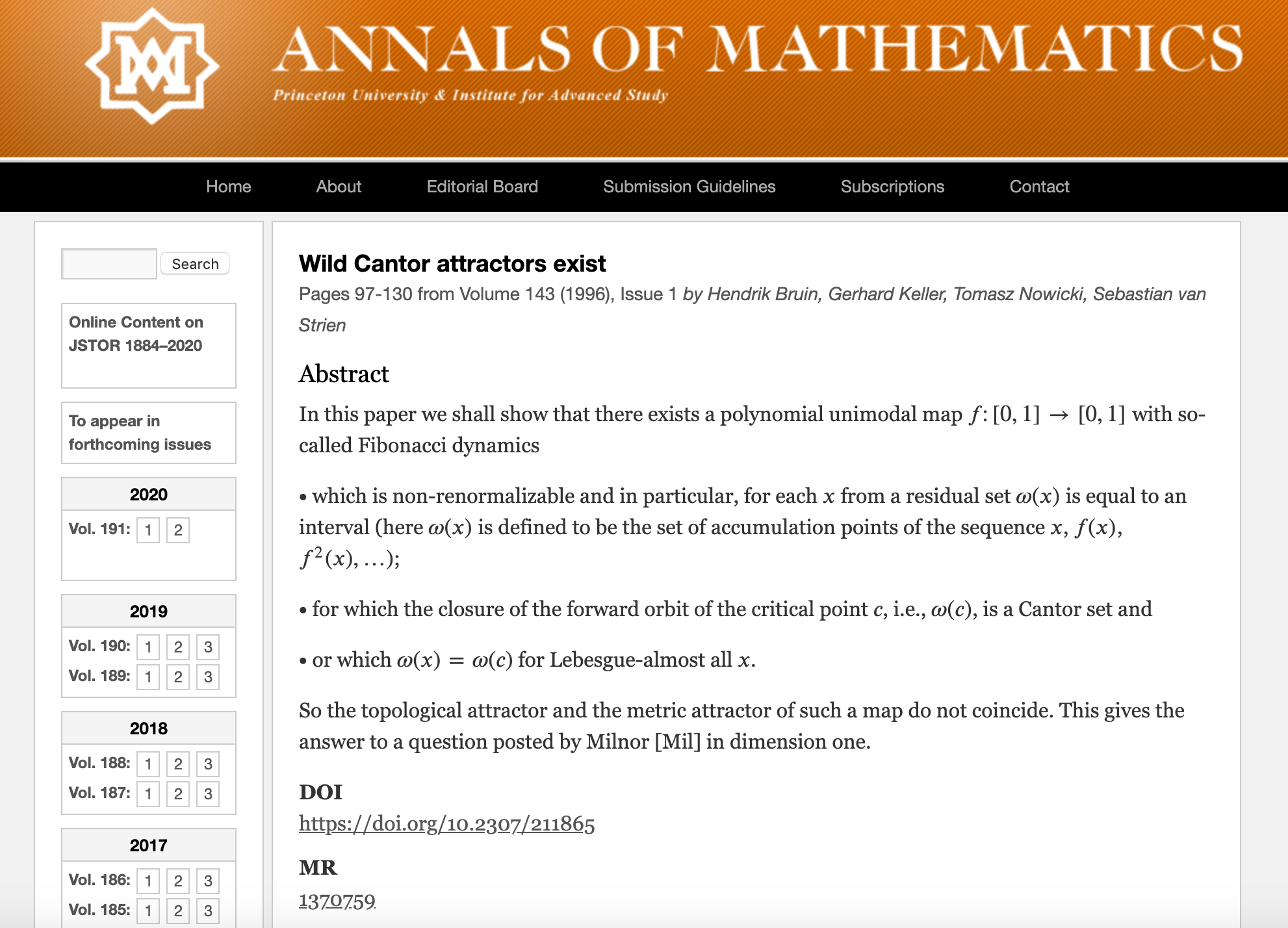
 do not have such Cantor attractors. Moreover, Lyubich has shown that these absorbing Cantor attractors can not exist if the critical point is quadratic. However, Bruin, Keller, Nowicki and Van Strien showed that the absorbing Cantor attractors exist for Fibonacci maps when the critical order
  is sufficiently large enough.
 unimodal, has a quadratic critical point, has negative Schwarzian derivative and has no periodic attractors, then each closed forward invariant set
  to be the maximal interval on which
  is monotone. Let
  and
and  be the components of
  and define
  be the minimum of the length of
  and
and  .
. for almost all
  of
of  such that for almost every
  of
of  is monotone,
  and
and  .
. or
or 
 is
is  , with a bound on the first and the second derivatives. Assume that the interval
 ![[q_{0},q_{k}]](https://s0.wp.com/latex.php?latex=%5Bq_%7B0%7D%2Cq_%7Bk%7D%5D&bg=ffffff&fg=2b2b2b&s=0&c=20201002) ( or
( or ![[q_{0},q_{\infty}]](https://s0.wp.com/latex.php?latex=%5Bq_%7B0%7D%2Cq_%7B%5Cinfty%7D%5D&bg=ffffff&fg=2b2b2b&s=0&c=20201002) ) is positive invariant, so
) is positive invariant, so ![f(x)\in [q_{0},q_{k}]](https://s0.wp.com/latex.php?latex=f%28x%29%5Cin+%5Bq_%7B0%7D%2Cq_%7Bk%7D%5D&bg=ffffff&fg=2b2b2b&s=0&c=20201002) for all
for all ![x\in [q_{0}, q_{k}]](https://s0.wp.com/latex.php?latex=x%5Cin+%5Bq_%7B0%7D%2C+q_%7Bk%7D%5D&bg=ffffff&fg=2b2b2b&s=0&c=20201002) ( or
( or ![f(x)\in [q_{0},q_{\infty}]](https://s0.wp.com/latex.php?latex=f%28x%29%5Cin+%5Bq_%7B0%7D%2Cq_%7B%5Cinfty%7D%5D&bg=ffffff&fg=2b2b2b&s=0&c=20201002) for all
for all ![x\in[q_{0},q_{\infty}]](https://s0.wp.com/latex.php?latex=x%5Cin%5Bq_%7B0%7D%2Cq_%7B%5Cinfty%7D%5D&bg=ffffff&fg=2b2b2b&s=0&c=20201002) ).
). ( or
( or  ),assume that we have defined densities up to
  , then define define
  as follows
 , which takes one density function to another function, is called the Perron-Frobenius operator. The limit of the first
  ,
,
 .
.
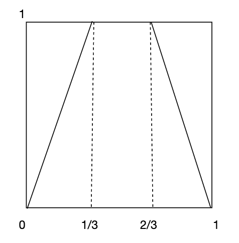
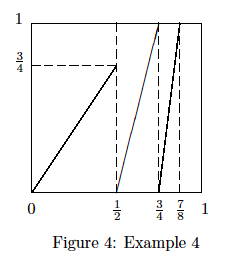
 on
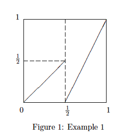
on ![[0,1]](https://s0.wp.com/latex.php?latex=%5B0%2C1%5D&bg=ffffff&fg=2b2b2b&s=0&c=20201002) . From the definition of
. From the definition of  , the slope on
  and
and  are 1 and 2, respectively. If
  , then it has only one pre-image on
  , then it has two pre-images, one is
  in
in  in
in 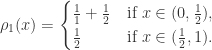


 , then


 . By induction,
  on
on  . Therefore,
  on
on 

 . By similar considerations,

 and
and  for all


 and
and  for all
![A=[a_{ij}]](https://s0.wp.com/latex.php?latex=A%3D%5Ba_%7Bij%7D%5D&bg=ffffff&fg=2b2b2b&s=0&c=20201002) be a
be a  matrix. We say
  for all
  . Such a matrix is called irreducible if for any pair
  such that
  where
where  is the
  th element of
  . The matrix
  such that no eigenvalue of
  .
. and a non-negative right (column) eigenvector
  .
. ,
,  all
all  ).
). .
. has the largest absolute value in the set of all eigenvalues of
  for all pairs
  . That means
  is a strictly positive
  be a compact interval. A
  map
map  is called Markov if there exists a finite or countable family
  of disjoint open intervals in
  has Lebesgue measure zero and there exist
  and
and  such that for each
  and each interval
  such that
  is contained in one of the intervals
  one has
 , then
  ;
; such that
  for each
  . Usually, we will denote the Lebesgue measure of a Borel set
  .
. be corresponding partition. Then there exists a
  invariant probability measure
  on the Borel sets of
  is uniformly bounded and Holder continuous. Moreover, for each
  one has
  for some
  for every Borel set
  .
. for each interval
 ![f_{a}(x)=ax(1-x), a\in[0,4]](https://s0.wp.com/latex.php?latex=f_%7Ba%7D%28x%29%3Dax%281-x%29%2C+a%5Cin%5B0%2C4%5D&bg=ffffff&fg=2b2b2b&s=1&c=20201002) ,
, ![f_{a}:[0,1]\rightarrow [0,1]](https://s0.wp.com/latex.php?latex=f_%7Ba%7D%3A%5B0%2C1%5D%5Crightarrow+%5B0%2C1%5D&bg=ffffff&fg=2b2b2b&s=1&c=20201002) .
.![\{ a\in[0,4]: f_{a} \text{ satisfies Axiom A} \}](https://s0.wp.com/latex.php?latex=%5C%7B+a%5Cin%5B0%2C4%5D%3A+f_%7Ba%7D+%5Ctext%7B+satisfies+Axiom+A%7D+%5C%7D&bg=ffffff&fg=2b2b2b&s=1&c=20201002) 是否在 [0,4] 中稠密?
是否在 [0,4] 中稠密? 满足 Axiom A


 和
和  不是拓扑共轭的,即使它们的 Kneading 序列是一样的。
 .
. 和
和  拓扑同胚,则有

 在这里
在这里  都是复平面上面的连通开集,
  是保持定向的同胚映射,称
  ), 如果
), 如果 是 ACL 的,也就是线段上绝对连续,absolutely continuous on lines.
 几乎处处成立。
 有
有
 几乎处处成立。
 则
则 

![a_{0} \in (0,4]](https://s0.wp.com/latex.php?latex=a_%7B0%7D+%5Cin+%280%2C4%5D&bg=ffffff&fg=2b2b2b&s=1&c=20201002)
![Comb(a_{0})=\{ a\in(0,4]: K(f_{a})=K(f_{a_{0}}) \},](https://s0.wp.com/latex.php?latex=Comb%28a_%7B0%7D%29%3D%5C%7B+a%5Cin%280%2C4%5D%3A+K%28f_%7Ba%7D%29%3DK%28f_%7Ba_%7B0%7D%7D%29+%5C%7D%2C&bg=ffffff&fg=2b2b2b&s=1&c=20201002)
![Top(a_{0})= \{ a\in (0,4]: f_{a} \text{ and } f_{a_{0}} \text{ are topological conjugate } \},](https://s0.wp.com/latex.php?latex=Top%28a_%7B0%7D%29%3D+%5C%7B+a%5Cin+%280%2C4%5D%3A+f_%7Ba%7D+%5Ctext%7B+and+%7D+f_%7Ba_%7B0%7D%7D+%5Ctext%7B+are+topological+conjugate+%7D+%5C%7D%2C&bg=ffffff&fg=2b2b2b&s=1&c=20201002)

![Qc(a_{0}) = \{ a\in (0,4]: f_{a} \text{ and } f_{a_{0}} \text{ are quasi-conformal conjugate} \},](https://s0.wp.com/latex.php?latex=Qc%28a_%7B0%7D%29+%3D+%5C%7B+a%5Cin+%280%2C4%5D%3A+f_%7Ba%7D+%5Ctext%7B+and+%7D+f_%7Ba_%7B0%7D%7D+%5Ctext%7B+are+quasi-conformal+conjugate%7D+%5C%7D%2C+&bg=ffffff&fg=2b2b2b&s=1&c=20201002)
![Aff(a_{0}) = \{ a\in (0,4]: f_{a} \text{ and } f_{a_{0}} \text{ are linear conjugate} \},](https://s0.wp.com/latex.php?latex=Aff%28a_%7B0%7D%29+%3D+%5C%7B+a%5Cin+%280%2C4%5D%3A+f_%7Ba%7D+%5Ctext%7B+and+%7D+f_%7Ba_%7B0%7D%7D+%5Ctext%7B+are+linear+conjugate%7D+%5C%7D%2C+&bg=ffffff&fg=2b2b2b&s=1&c=20201002)

 没有双曲吸引或者中性周期轨,则
![f:[0,1]\rightarrow [0,1]](https://s0.wp.com/latex.php?latex=f%3A%5B0%2C1%5D%5Crightarrow+%5B0%2C1%5D+&bg=ffffff&fg=2b2b2b&s=1&c=20201002) 是
是  ,
,  是正整数,则存在
![f_{n}:[0,1]\rightarrow [0,1]](https://s0.wp.com/latex.php?latex=f_%7Bn%7D%3A%5B0%2C1%5D%5Crightarrow+%5B0%2C1%5D&bg=ffffff&fg=2b2b2b&s=0&c=20201002) 使得
使得 ![|| f_{n}- f ||_{C^{k}}=\max_{x\in[0,1]} \max_{0\leq m\leq k} |D^{m}f_{n}(x)-D^{m}f(x)| \rightarrow 0](https://s0.wp.com/latex.php?latex=%7C%7C+f_%7Bn%7D-+f+%7C%7C_%7BC%5E%7Bk%7D%7D%3D%5Cmax_%7Bx%5Cin%5B0%2C1%5D%7D+%5Cmax_%7B0%5Cleq+m%5Cleq+k%7D+%7CD%5E%7Bm%7Df_%7Bn%7D%28x%29-D%5E%7Bm%7Df%28x%29%7C+%5Crightarrow+0&bg=ffffff&fg=2b2b2b&s=1&c=20201002) as
as  , 这里的每个
 都满足Axiom A。
 是紧致度量空间,
 是连续函数。如果
 是使得
是使得 的最小正整数,则称x是以n为周期的周期点。
 .
. ,
, ,
, i.e.
i.e. ![X=[0,1]](https://s0.wp.com/latex.php?latex=X%3D%5B0%2C1%5D&bg=ffffff&fg=2b2b2b&s=1&c=20201002) ,
, ![f(x)\in C^{1}[0,1]](https://s0.wp.com/latex.php?latex=f%28x%29%5Cin+C%5E%7B1%7D%5B0%2C1%5D&bg=ffffff&fg=2b2b2b&s=1&c=20201002) ,
,  是以n为周期的周期轨道, 定义乘子(multiplier)
  。
。 称为
称为 是双曲周期轨。
 称为中性周期轨。
 称为双曲吸引轨。
 称为双曲斥性轨。
![f:[0,1]\rightarrow [0,1]](https://s0.wp.com/latex.php?latex=f%3A%5B0%2C1%5D%5Crightarrow+%5B0%2C1%5D&bg=ffffff&fg=2b2b2b&s=1&c=20201002) 是
是 映射,A是紧集并且
 使得对任意的
 , 有
, 有 ,则称A是双曲集。
 ,
, 是双曲吸引轨
  的吸引区域,
 ![\Omega=[0,1]\setminus \cup_{i=1}^{m}B(\theta_{i})](https://s0.wp.com/latex.php?latex=%5COmega%3D%5B0%2C1%5D%5Csetminus+%5Ccup_%7Bi%3D1%7D%5E%7Bm%7DB%28%5Ctheta_%7Bi%7D%29&bg=ffffff&fg=2b2b2b&s=1&c=20201002) 是双曲集。
是双曲集。 ,1是双曲斥性不动点,0是双曲吸引不动点。
 ,
, ![\Omega=[-1,1]\setminus B(\{0\})=\{-1,1\}](https://s0.wp.com/latex.php?latex=%5COmega%3D%5B-1%2C1%5D%5Csetminus+B%28%5C%7B0%5C%7D%29%3D%5C%7B-1%2C1%5C%7D&bg=ffffff&fg=2b2b2b&s=1&c=20201002) .
.  ,
,  . 取
. 取 .
. .
. 并且
并且 . i.e.
  是
是 连续的,
连续的, 如果A是双曲集,则A的Lebesgue测度是零。
 的映射,
的映射, , 则存在双曲吸引周期轨
  使得
使得 
 f 满足 Axiom A。
 ,
,![\Lambda_{U} = \{ x\in[0,1]: f^{n}(x)\notin U, \forall n\geq 0 \}](https://s0.wp.com/latex.php?latex=%5CLambda_%7BU%7D+%3D+%5C%7B+x%5Cin%5B0%2C1%5D%3A+f%5E%7Bn%7D%28x%29%5Cnotin+U%2C+%5Cforall+n%5Cgeq+0+%5C%7D&bg=ffffff&fg=2b2b2b&s=1&c=20201002) ,
,
 是双曲集。
是双曲集。 be intervals and let l, r be the components of
  . Then the Cross Ratio is defined as


 for some
  and
and  , then
  for all
  .
.![I=[a,b]](https://s0.wp.com/latex.php?latex=I%3D%5Ba%2Cb%5D&bg=ffffff&fg=2b2b2b&s=0&c=20201002) ,
,  is a
is a 
 and any n for which
  is a diffeomorphism one has the following. If
  contains a
  scaled neighbourhood of
  , then
 which does not depend on f, n, and t such that
 contains a
  . Then for any univalent function
  one has a universal function
  such that
 is the unit disc on the complex plane
  ,
,  is a holomorphic function with
  . Then
  for all
  and
and  Moreover, if
  for some
  or
or  then
then  for some
 is the unit disc on the complex plane
  is a holomorphic function, then

 is the upper half plane of the complex plane
  is a holomorphic map. Then
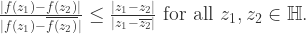

 , assume
  denotes the hyperbolic distance between
  and
and  on
on 
 for some points
  , then
  , where

 is an interval. It is easy to show that
  is conformally equivalent to the upper half plane and define
  as
as
 at which the discs intersect the real line. Moreover,
  Define
 is a holomorphic map, then
 is a real polynomial map, its critical points are on the real line. Assume
  is a diffeomorphism, then there exists a set
  such that
  and
and is a conformal map.
 and assume f maps the real line to the real line. For each
  there exists
  such that if J is a real interval in
  , then
 is
is

 is
is
 , then the hyperbolic length of the interval
  on the total interval
  is
is

 is a
is a  , then

 be a
be a  , then there exists a unique
  such that
  for all
  . Therefore, assume that
  or
or  for all
  . Since
  is a continuous function on the closed interval I, there exists
 such that
  for all
  .
. such that
  . Since the schwarzian derivative of
 . However, from the definition of
  , we get


 , there exists
  such that, if
 ![f: [-\tau, 1+\tau] \rightarrow \mathbb{R}](https://s0.wp.com/latex.php?latex=f%3A+%5B-%5Ctau%2C+1%2B%5Ctau%5D+%5Crightarrow+%5Cmathbb%7BR%7D&bg=ffffff&fg=2b2b2b&s=0&c=20201002) is a
is a  for all
 ![t\in [-\tau,1+\tau],](https://s0.wp.com/latex.php?latex=t%5Cin+%5B-%5Ctau%2C1%2B%5Ctau%5D%2C&bg=ffffff&fg=2b2b2b&s=0&c=20201002) then we have
then we have
 Show that
  as
as  (This recovers the classical Koebe non-linearity principle).