Normal Families

October 20, 2014 zr9558 Leave a comment

Reference Book: Joel L.Schiff- Normal Families

Some Classical Theorems

Weierstrass Theorem Let $\{ f_{n}\}$ be a sequence of analytic functions on a domain $\Omega$ which converges uniformly on compact subsets of $\Omega$ to a function $f$ . Then $f$ is analytic in $\Omega$ , and the sequence of derivatives $\{ f_{n}^{(k)}\}$ converges uniformly on compact subsets to $f^{(k)}, k=1,2,3...$ .

Hurwitz Theorem Let $\{ f_{n}\}$ be a sequence of analytic functions on a domain $\Omega$ which converges uniformly on compact subsets of $\Omega$ to a non-constant analytic function $f(z)$ . If $f(z_{0})=0$ for some $z_{0}\in\Omega$ , then for each $r>0$ sufficiently small, there exists an $N=N(r)$ , such that for all $n>N$ , $f_{n}(z)$ has the same number of zeros in $D(z_{0},r)$ as does $f(z)$ . (The zeros are counted according to multiplicity).

The Maximum Principle If $f(z)$ is analytic and non-constant in a region $\Omega$ , then its absolute value $|f(z)|$ has no maximum in $\Omega$ .

The Maximum Principle’ If $f(z)$ is defined and continuous on a closed bounded set $E$ and analytic on the interior of $E$ , then the maximum of $|f(z)|$ on $E$ is assumed on the boundary of $E$ .

Corollary 1.4.1 If $\{ f_{n}\}$ is a sequence of univalent analytic functions in a domain $\Omega$ which converge uniformly on compact subsets of $\Omega$ to a non-constant analytic function $f$ , then $f$ is univalent in $\Omega$ .

Definition 1.5.1 A family of functions $\mathcal{F}$ is locally bounded on a domain $\Omega$ if, for each $z_{0}\in \Omega$ , there is a positive number $M=M(z_{0})$ and a neighbourhood $D(z_{0},r)\subset \Omega$ such that $|f(z)|\leq M$ for all $z\in D(z_{0}, r)$ and all $f\in \mathcal{F}$ .

Theorem 1.5.2 If $\mathcal{F}$ is a family of locally bounded analytic functions on a domain $\Omega$ , then the family of derivatives $\mathcal{F}^{'}=\{ f^{'}: f\in \mathcal{F}\}$ form a locally bounded family in $\Omega$ .

The converse of Theorem 1.5.2 is false, since $\mathcal{F}=\{n: n=1,2,3...\}$ . However, the following partial converse does hold.

Theorem 1.5.3 Let $\mathcal{F}$ be a family of analytic functions on $\Omega$ such that the family of derivatives $\mathcal{F}^{'}$ is locally bounded and suppose that there is some $z_{0}\in \Omega$ with $|f(z_{0})|\leq M<\infty$ for all $f\in \mathcal{F}$ . Then $\mathcal{F}$ is locally bounded. (Hint: find a path connecting $z_{0}$ and $z$ .)

Definition 1.6.1 A family $\mathcal{F}$ of functions defined on a domain $\Omega$ is said to be equicontinuous (spherically continuous) at a point $z^{'}\in \Omega$ if, for each $\epsilon>0$ , there is a $\delta=\delta(\epsilon,z^{'})>0$ such that $|f(z)-f(z^{'})|<\epsilon$ , $(\chi(f(z),f(z^{'}))<\epsilon)$ whenever $|z-z^{'}|<\delta$ , for every $f\in \mathcal{F}$ . Moreover, $\mathcal{F}$ is equicontinuous (spherical continuous) on a subset $E\subset \Omega$ if it is continuous (spherically continuous) at each point of $E$ .

Normal Families of Analytic Functions

Definition 2.1.1 A familiy $\mathcal{F}$ of analytic functions on a domain $\Omega\subset \mathbb{C}$ is normal in $\Omega$ if every sequence of functions $\{f_{n}\}\subset \mathcal{F}$ contains either a subsequence which converges to a limit function $f\not\equiv \infty$ uniformly on each compact subset of $\Omega$ , or a subsequence which converges uniformly to $\infty$ on each compact subset.

The family $\mathcal{F}$ is said to be normal at a point $z_{0}\in\Omega$ if it is normal in some neighbourhood of $z_{0}$ .

Theorem 2.1.2 A family of analytic functions $\mathcal{F}$ is normal in a domain $\Omega$ if and only if $\mathcal{F}$ is normal at each point in $\Omega$ .

Theorem 2.2.1 Arzela-Ascoli Theorem. If a sequence $\{f_{n}\}$ of continuous functions converges uniformly on a compact set $K$ to a limit function $f\not\equiv \infty$ , then $\{f_{n}\}$ is equicontinuous on $K$ , and $f$ is continuous. Conversely, if $\{f_{n}\}$ is equicontinuous and locally bounded on $\Omega$ , then a subsequence can be extracted from $\{f_{n}\}$ which converges locally uniformly in $\Omega$ to a (continuous) limit function $f$ .

Montel’s Theorem If $\mathcal{F}$ is a locally bounded family of analytic functions on a domain $\Omega$ , then $\mathcal{F}$ is a normal family in $\Omega$ .

Koebe Distortion Theorem Let $f(z)$ be analytic univalent in a domain $\Omega$ and $K$ a compact subset of $\Omega$ . Then there exists a constant $c=c(\Omega, K)$ such that for any $z,w\in K$ , $c^{-1}\leq |f^{'}(z)| / |f^{'}(w)| \leq c$ .

Vitali-Porter Theorem Let $\{f_{n}\}$ be a locally bounded sequence of analytic functions in a domain $\Omega$ such that $\lim_{n\rightarrow \infty}f_{n}(z)$ exists for each $z$ belonging to a set $E\subset \Omega$ which has an accumulation point in $\Omega$ . Then $\{ f_{n}\}$ converges uniformly on compact subsets of $\Omega$ to an analytic function.

Proof. From Montel’s Theorem, $\{ f_{n}\}$ is normal, extract a subsequence $\{ f_{n_{k}}\}$ which converges normally to an analytic function $f$ . Then $\lim_{k\rightarrow \infty} f_{n_{k}}(z)=f(z)$ for each $z\in E$ . Suppose, however, that $\{ f_{n}\}$ does not converge uniformly on compact subsets of $\Omega$ to $f$ . Then there exists some $\epsilon>0$ , a compact subset $K\subset \Omega$ , as well as a subsequence $\{f_{m_{j}}\}$ and points $z_{j}\in K$ satisfying $|f_{m_{j}}(z_{j})- f(z_{j})| \geq \epsilon,$ $j=1,2,3,...$ . Now $\{ f_{m_{j}}\}$ itself has a subsequence which converges uniformly on compact subsets to an analytic function $g$ , and $g\not\equiv f$ from above. However, since $f$ and $g$ must agree at all points of $E$ , the Identity Theorem for analytic functions implies $f\equiv g$ on $\Omega$ , a contradiction which establishes the theorem.

Fundamental Normality Test Let $\mathcal{F}$ be the family of analytic functions on a domain $\Omega$ which omit two fixed values $a$ and $b$ in $\mathbb{C}$ . Then $\mathcal{F}$ is normal in $\Omega$ .

Generalized Normality Test Suppose that $\mathcal{F}$ is a family of analytic functions in a domain $\Omega$ which omit a value $a\in \mathbb{C}$ and such that no function of $\mathcal{F}$ assumes the value $b\in \mathbb{C}$ at more that $p$ points. Then $\mathcal{F}$ is normal in $\Omega$ .

2.3 Examples:

Assume $U$ is the unit disk in the complex plane, $\Omega$ is a region (connected open set) in $\mathbb{C}$ .

1. $\mathcal{F}=\{ f_{n}(z)=z^{n}: n=1,2,3...\}$ in $U$ . Then $\mathcal{F}$ is normal in $U$ , but not compact since $0 \notin \mathcal{F}$ . In the domain $U^{'}: |z|>1$ , $\mathcal{F}$ is normal.

2. $\mathcal{F}=\{ f_{n}(z)=\frac{z}{n}: n=1,2,3...\}$ is a normal family in $\mathcal{C}$ but not compact.

3. $\mathcal{F}=\{ f: f$ analytic in $\Omega$ and $|f|\leq M \}$ . Then $\mathcal{F}$ is normal in $\Omega$ and compact.

4. $\mathcal{F}=\{ f: f$ analytic in $\Omega$ and $\Re f>0\}$ . Then $\mathcal{F}$ is normal but not compact. Hint: $\mathcal{G}=\{g=e^{-f}:f\in \mathcal{F}\}$ is a uniformly bounded family.

5. $\mathcal{S}=\{ f: f$ analytic, univalent in $U$ , $f(0)=0, f^{'}(0)=1 \}$ . These are the normalised “Schlicht” functions in $U$ . $\mathcal{S}$ is normal and compact.

Normal Families of Meromorphic Functions

Assume a function $f(z)$ is analytic in a neighbourhood of $a$ , except perhaps at $a$ itself. In other words, $f(z)$ shall be analytic in a region $0<|z-a|<\delta$ . The point $a$ is called an isolated singularity of $f(z)$ . There are three cases about an isolated singularity. The first one is a removable singularity, the second one is a pole, the third one is an essential singularity. A function $f(z)$ which is analytic in a region $\Omega$ , except for poles, is said to be meromorphic in $\Omega$ .

The chordal distance $\chi(z_{1}, z_{2})$ between $z_{1}$ and $z_{2}$ is

$\chi(z_{1}, z_{2}) = \frac{|z_{1}-z_{2}|}{\sqrt{1+|z_{1}|^{2}}\sqrt{1+|z_{2}|^{2}}}$ if $z_{1}$ and $z_{2}$ are in the finite plane, and

$\chi(z_{1}, \infty) = \frac{1}{\sqrt{1+|z_{1}|^{2}}},$ if $z_{2}=\infty$ . Clearly, $\chi(z_{1}, z_{2})\leq 1$ , and $\chi(z_{1}^{-1}, z_{2}^{-1}) = \chi(z_{1}, z_{2})$ . The chordal metric and spherical metric are uniformly equivalent and generate the same open sets on the Riemann sphere.

Definition 1.2.1 A sequence of functions $\{ f_{n}\}$ converges spherically uniformly to $f$ on a set $E\subset \mathbb{C}$ if, for any $\epsilon>0$ , there is a number $n_{0}$ such that $n\geq n_{0}$ implies $\chi(f(z), f_{n}(z))<\epsilon$ , for all $z\in E$ .

Definition 3.1.1 A family $\mathcal{F}$ of meromorphic functions in a domain $\Omega$ is normal in $\Omega$ if every sequence $\{ f_{n} \} \subset \mathcal{F}$ contains a subsequence which converges spherically uniformly on compact subsets of $\Omega$ .

Theorem 3.1.3 Let $\{ f_{n}\}$ be a sequence of meromorphic functions on a domain $\Omega$ . Then $\{ f_{n}\}$ converges spherically uniformly on compact subsets of $\Omega$ to $f$ if and only if about each point $z_{0}\in \Omega$ there is a closed disk $K(z_{0},r)$ in which $|f_{n}-f|\rightarrow 0$ or $|1/f_{n} - 1/f| \rightarrow 0$ uniformly as $n\rightarrow \infty$ .

Corollary 3.1.4 Let $\{ f_{n}\}$ be a sequence of meromorphic functions on $\Omega$ which converges spherically uniformly on compact subsets to $f$ . Then $f$ is either a meromorphic function on $\Omega$ or identically equal to $\infty$ .

Corollary 3.1.5 Let $\{ f_{n}\}$ be a sequence of analytic functions on a domain $\Omega$ which converge spherically uniformly on compact subsets of $\Omega$ to $f$ . Then $f$ is either analytic on $\Omega$ or identically equal to $\infty$ .

Theorem 3.2.1 A family $\mathcal{F}$ of meromorphic functions in a domain $\Omega$ is normal if and only if $\mathcal{F}$ is spherically equicontinuous in $\Omega$ .

Fundamental Normality Test Let $\mathcal{F}$ be a family of meromorphic functions on a domain $\Omega$ which omit three distinct values $a, b, c \in \mathbb{C}$ . Then $\mathcal{F}$ is normal in $\Omega$ .

Vitali-Porter Theorem Let $\{f_{n}\}$ be a sequence belonging to a spherically equicontinuous family of meromorphic functions such that $\{ f_{n}(z)\}$ converges spherically on a point set $E$ having an accumulation point in $\Omega$ . Then $\{ f_{n}\}$ converges spherically uniformly on compact subsets of $\Omega$ .

Let $f(z)$ be meromorphic on a domain $\Omega$ . If $z\in \Omega$ is not a pole, the derivative in the spherical metric, called the spherical derivative, is given by 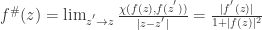$f^{\#}(z) =\lim_{z^{'}\rightarrow z}\frac{\chi(f(z),f(z^{'}))}{|z-z^{'}|} =\frac{|f^{'}(z) |}{1+|f(z)|^{2}}$ . If $\zeta$ is a pole of $f(z)$ , define $f^{\#}(\zeta) = \lim_{z\rightarrow \zeta} \frac{|f^{'}(z)|}{1+|f(z)|^{2}}$ .

Marty’s Theorem A family $\mathcal{F}$ of meromorphic functions on a domain $\Omega$ is normal if and only if for each compact subset $K\subset \Omega$ , there exists a constant $C=C(K)$ such that spherical derivative $f^{\#}(z) =\frac{|f^{'}(z) |}{1+|f(z)|^{2}}\leq C, z\in K, f\in \mathcal{F},$ that is, $f^{\#}$ is locally bounded.

数学界的八卦

[转载]痛批计算数学所

October 13, 2014 zr9558 Leave a comment

发信人: rodm48gmf (—>—>—>—>—>—>—>—>—>—),

信区: D_Maths

标题: 老板痛批计算数学所（转）

发信站: 南京大学小百合站 (Sat Oct 11 15:59:23 2014)

昨天讨论班上，一位师兄就博士论文向老板咨询。老板语重心长的说：现在好歹也是博士了，论文里必须要有些自己的东西，能拿别人的东西拼凑！接着话锋一转，说道：最近中国的大飞机搞得很热闹，发动机是别人的不算，连自己测试出来的飞机模型数据因为没有算法也不会算，只好花了6000万美金问老美买软件。但美方条件相当苛刻，要求中方把初始数据的备份拷给美方，等美方分析完了，再把最终结果告诉你，中间过程没法看到。这下可好，不但算法核心没法掌握，连同我们的飞机性能也让人家了如指掌了，不用侦查卫星，就把你查个底朝天。

老板接着说：回头看我们的计算数学所，近几年来对数学理论本身的要求越来越弱化。招的学生在本科就学些计算数学专业的数值分析，数学软件。到了研究生阶段，只看见天天泡在电脑前面敲键盘、调试程序，写出的算法无非是对已有的东西小打小闹，根本没有理论深度。也不是他不花功夫，是实在是层次太低，别说微分几何、代数拓扑这些常规的东西都不懂，即使是本科的数学物理方程，真正学好的人也没几个。对偏微分方程的认识皮毛也谈不上，你说他怎么写的出好的算法。

老板还说，若把那些大飞机、卫星项目让企业来做，就更加不行了。那些工程师自从高校中出去以后，就开始吃老本，天下算法一大抄，有的甚至为了拟合精度而篡改实验数据，这样造出来的飞机、卫星能不掉下来吗？当然为了混口饭吃，这么做也并不难理解。

最后，老板说道：反观数学所，我们也没必要高兴到哪里去。可能我们这儿招的做PDE的学生，数学物理方程还没计算所的好呢。现在国家急了，对重大计算项目特别重视，基金委拨了2亿元立项，十二五期间务必在这方面有重大突破。所以啊，不管怎么说，大家做东西一定得有自己的想法，一步步把结果做上去！现在无论是做大飞机、还是搞卫星，都需要研究人员不仅会编写程序，还要懂得其中深刻的数学原理，可能它的理论难点就涉及某些奇点理论，这就需要大家懂微分几何、懂流形拓扑、懂奇点理论。物理背景的重要性是毋庸置疑的，量子理论作为物理的两大基石之一，处处发挥重要作用。如果我们的研究人员都具备了这样的素质，我们的科研才有希望。而中国的计算数学差就差在两点：一、没有数学理论做依托，只会微积分和矩阵论。二、系统集成能力太差，编出Windows之类的操作系统根本不可能！

※ 来源:．南京大学小百合站 http://bbs.nju.edu.cn

[FROM: 114.212.206.39]

MA 1505 Mathematics I

Prediction of Final Exam 2014-2015 Semester I

October 12, 2014 zr9558 Leave a comment

Module: MA 1505 Mathematics I

Time: 2 hours ( 120 minutes ), Saturday, 22-Nov-2014 (Morning)

Questions: 8 questions, each question contains two questions. i.e. 16 questions.

Average speed: 7.5 minutes per question.

Scores: 20% mid-term exam, 80% final exam. i.e. Each question in the final exam is 5%.

Remark: Another Possibility: 5 Chapters, each chapter contains 1 big question, and each question contains three small questions, i.e. 15 questions. 8 minutes per question.

The contents in high school:

Trigonometric functions, some basic inequalities and identities.

The contents before mid-term exam: Please review the details of them.

Chapter 2: Differentiation

Derivatives of one variable functions, derivatives of parameter functions, Chain rule of derivatives, the tangent line of the curve, L.Hospital Rule, critical points of one variable, local maximum and local minimum of one variable function.

Chapter 3: Integration

Integration by parts, Newton-Leibniz Formula, the area of the domain in the plane, the volume of the solid which is generated by a curve rotated with an axis.

Chapter 4: Series

Taylor Series and Power Series, radius of convergence of power series, the convergence domain of power series, the sum of geometric series and arithmetic series.

Chapter 5: Three Dimensional Spaces

Cross Product and Dot Product of vectors, projection of vectors, the equation of the plane and the line in 3-dimensional space, Distance from a point to a plane, Distance from a point to a line, the distance between two lines in two or three dimensional spaces, the distance between two parallel planes. Intersection points of two different curves.

The contents after mid-term exam: Must prepare them.

By the way, 2-3 questions means at least 2 questions, at most 3 questions. 0-1 question means 0 question or 1 question.

Geometric Graphs in Three Dimensional Space:

http://www.wolframalpha.com

$z=x^{2}+y^{2},$ $z=-(x^{2}+y^{2})$ infinite paraboloid

$z=x^{2}-y^{2}$ hyperbolic paraboloid

$(x-x_{0})^{2}+(y-y_{0})^{2}+(z-z_{0})^{2}=R^{2}$ sphere with radius $R>0$ and center $(x_{0},y_{0},z_{0})$

$x^{2}+y^{2}=R^{2},$ $y^{2}+z^{2}=R^{2},$ $z^{2}+x^{2}=R^{2}$ cylinder

$ax+by+cz=d, \text{ where } a,b,c,d \in \mathbb{R}$ Plane

$y=x^{2}+c \text{ and } x=y^{2}+c, \text{ where } c\in \mathbb{R}$ Parabola

Chapter 6: Fourier Series:

Fourier Coefficients of functions with period $2\pi$ : 1 question. Especially, $a_{2014}$ and $b_{2014}$ (Integration by parts).

Fourier Coefficients of functions with period $2L$ : 1 question, where $L$ is a positive real number. Especially, $a_{2014}$ and $b_{2014}$ (Integration by parts).

Calculate the summation of Fourier coefficients: 0-1 question. Especially, $\sum_{n=0}^{\infty} a_{n}$ and $\sum_{n=1}^{\infty} a_{n}$ .

Cosine and sine expansion of function on the half domain: 1 question.

Chapter 7: Function of Several Real Variables

Directional derivatives, partial derivatives, gradient of functions with two or three variables, Chain Rule of partial derivatives: 1-2 questions. (Pay attention to whether the vector is a unit vector or not. If it is not a unit vector, you should change it to a unit vector first, and then calculate the directional derivatives).

Critical points of two variable functions (saddle point, local maximum, local minimum): 0-1 question. (Calculate the partial derivatives first, then evaluate the critical points, so we can decide the property of the critical points from some rules).

Lagrange’s method: 0-1 question. (Calculate the maximum value of functions under some special conditions. Construct the function first, evaluate partial derivatives secondly, and calculate the critical points of the new functions. In addition, if you use inequality “arithmetic mean” is greater than “geometric mean”, then the question will become easier.)

Chapter 8: Multiple Integral

Double integral, polar coordinate: 1 question. (The formula of polar coordinate in the plane).

Reverse the order of integration of double integral: 1 question. (Draw the picture of domain $R$ and reverse the order of dx and dy).

Volume of the solid: 1 question. (Double integral, find the function $z=z(x,y)$ and the domain $R$ on the $xy-$ plane. If the domain $R$ is a disk or a sector, then you can use the polar coordinate).

Area of the surface: 1 question. (Partial Derivatives of functions with two variables, the domain $R$ on the $xy-$ plane. If the domain $R$ is a disk or a sector, then you can use the polar coordinate. The area of a surface is a special case of the surface integral of a scalar field).

Triple integral: 0-1 question. (The method to calculate the triple integral is similar to double integral).

Chapter 9: Line Integrals

Length of a curve: 0-1 question. (Parameter equation of the curves. Length of a curve is a special case of line integral of a scalar field).

Line integrals of scalar fields: 1 question. (The equation of line segment, the equation of the circle with radius $R$ , the length of vectors). Geometric meaning: the area of the wall along the curve.

Line integrals of vector fields: 1 question. (The equation of line segments, the equation of the circle with radius $R$ , Dot product of vectors). Physical meaning: Work done.

Conservative vector fields and Newton-Leibniz formula of gradient vector fields: 0-1 question. (Definition of conservative vector field and its equivalent condition. When the value of a line integral of vector field is independent to the curve $C$ , where $C$ has the fixed initial point and the terminal point?).

Green’s Theorem: 1 question. (Two cases: the boundary is open; the boundary is closed. If the curve is open, you should close it by yourself.) Pay attention to the orientation, i.e. anticlockwise and left hand rule.

Chapter 10: Surface Integrals

Tangent plain of a surface: 0-1 question. (Partial derivatives, Cross product of two vectors, Normal vector of a plane)

Surface integrals of scalar fields: 1 question. (The equation of surface $z=z(x,y)$ and the projection of the surface on the $xy-$ plane, Cross product of vectors, the length of vectors. Change the surface integrals of scalar fields to double integrals).

Surface integrals of vector fields: 1 question. (The equation of surface $z=z(x,y)$ and the projection of the surface on the $xy-$ plane, Cross product and Dot product of vectors).

Stokes’ Theorem: 1 question. (This is a rule on line integrals of vector fields and surface integrals of vector fields. Remember the operator $curl$ . Pay attention to the orientation of the curve on the boundary, i.e. the right hand rule).

Divergence Theorem: 0-1 question. (This is a rule on surface integrals of vector fields and triple integrals. Remember the operator $div$ ).

MA 1505 Mathematics I

Prediction of Middle Term Test

October 12, 2014 zr9558 Leave a comment

Module: MA 1505 Mathematics I

Time: 1 hours ( 60 minutes )

Questions: 10 Multiple Choice Questions.

Average speed: 6 minutes per question.

Scores: 20% in final score.

The contents in high school:

Trigonometric functions, some basic inequalities and identities.

Questions in middle term test:

Question 1. Derivatives, Tangent line of a function, Intersection point of tangent line and x-axis, y-axis. Basic Rules of differentiation, Chain Rule.

Question 2. Critical points of a function, how to calculate the maximum and minimum value of a function.

Question 3. Integration by parts, integrate trigonometric functions.

Question 4. Fundamental theorem of calculus.

Question 5. Find the area which is bounded by some curves.

Question 6. Mathematical models. ( e.g. light and ball drop, ship and so on).

Question 7. Radius of convergence of a power series, the interval of convergence of a power series.

Question 8. Calculate the Taylor series of functions, Calculate the coefficients of Taylor series.

Question 9. How to use Taylor series to calculate the solution of an equation.

Question 10. How to use Taylor series to calculate the summation of some series. ( Integration and differentiation).

Question 11. The length of a curve, the tangent line of a curve.

Question 12. Dot product and cross product of two vectors, equation of planes, normal vector of a plane, distance between a point and a plane.

ZHANG RONG

Monthly Archives: October 2014

Normal Families

Some Classical Theorems

Normal Families of Analytic Functions

Normal Families of Meromorphic Functions

[转载]痛批计算数学所

Prediction of Final Exam 2014-2015 Semester I

The contents in high school:

The contents before mid-term exam: Please review the details of them.

Chapter 2: Differentiation

Chapter 3: Integration

Chapter 4: Series

Chapter 5: Three Dimensional Spaces

The contents after mid-term exam: Must prepare them.

Geometric Graphs in Three Dimensional Space:

Chapter 6: Fourier Series:

Chapter 7: Function of Several Real Variables

Chapter 8: Multiple Integral

Chapter 9: Line Integrals

Chapter 10: Surface Integrals

Prediction of Middle Term Test

The contents in high school:

Questions in middle term test:

zr9558's Blog