异常点检测（又称为离群点检测）是找出其行为很不同于预期对象的一个检测过程。这些对象被称为异常点或者离群点。异常点检测在很多实际的生产生活中都有着具体的应用，比如信用卡欺诈，工业损毁检测，图像检测等。

本文主要介绍一些常见的异常点检测算法，包括基于统计的模型，基于距离的模型，线性变换的模型，非线性变换的模型等。

异常点检测和聚类分析是两项高度相关的人物。聚类分析发现数据集中的各种模式，而异常点检测则是试图捕捉那些显著偏离多数模式的异常情况。异常点检测和聚类模型服务于不同的目的。

This slideshow requires JavaScript.

Introduction

If things don’t go your way in predictive modeling, use XGboost.  XGBoost algorithm has become the ultimate weapon of many data scientist. It’s a highly sophisticated algorithm, powerful enough to deal with all sorts of irregularities of data.

Building a model using XGBoost is easy. But, improving the model using XGBoost is difficult (at least I struggled a lot). This algorithm uses multiple parameters. To improve the model, parameter tuning is must. It is very difficult to get answers to practical questions like – Which set of parameters you should tune ? What is the ideal value of these parameters to obtain optimal output ?

This article is best suited to people who are new to XGBoost. In this article, we’ll learn the art of parameter tuning along with some useful information about XGBoost. Also, we’ll practice this algorithm using a  data set in Python.

 

What should you know ?

XGBoost (eXtreme Gradient Boosting) is an advanced implementation of gradient boosting algorithm. Since I covered Gradient Boosting Machine in detail in my previous article – Complete Guide to Parameter Tuning in Gradient Boosting (GBM) in Python, I highly recommend going through that before reading further. It will help you bolster your understanding of boosting in general and parameter tuning for GBM.

Special Thanks: Personally, I would like to acknowledge the timeless support provided by Mr. Sudalai Rajkumar (aka SRK), currently AV Rank 2. This article wouldn’t be possible without his help. He is helping us guide thousands of data scientists. A big thanks to SRK!

 

Table of Contents

1. The XGBoost Advantage
2. Understanding XGBoost Parameters
3. Tuning Parameters (with Example)

 

1. The XGBoost Advantage

I’ve always admired the boosting capabilities that this algorithm infuses in a predictive model. When I explored more about its performance and science behind its high accuracy, I discovered many advantages:

1. Regularization:
   • Standard GBM implementation has no regularization like XGBoost, therefore it also helps to reduce overfitting.
   • In fact, XGBoost is also known as ‘regularized boosting‘ technique.
2. Parallel Processing:
   • XGBoost implements parallel processing and is blazingly faster as compared to GBM.
   • But hang on, we know that boosting is sequential process so how can it be parallelized? We know that each tree can be built only after the previous one, so what stops us from making a tree using all cores? I hope you get where I’m coming from. Check this link out to explore further.
   • XGBoost also supports implementation on Hadoop.
3. High Flexibility
   • XGBoost allow users to define custom optimization objectives and evaluation criteria.
   • This adds a whole new dimension to the model and there is no limit to what we can do.
4. Handling Missing Values
   • XGBoost has an in-built routine to handle missing values.
   • User is required to supply a different value than other observations and pass that as a parameter. XGBoost tries different things as it encounters a missing value on each node and learns which path to take for missing values in future.
5. Tree Pruning:
   • A GBM would stop splitting a node when it encounters a negative loss in the split. Thus it is more of a greedy algorithm.
   • XGBoost on the other hand make splits upto the max_depth specified and then start pruningthe tree backwards and remove splits beyond which there is no positive gain.
   • Another advantage is that sometimes a split of negative loss say -2 may be followed by a split of positive loss +10. GBM would stop as it encounters -2. But XGBoost will go deeper and it will see a combined effect of +8 of the split and keep both.
6. Built-in Cross-Validation
   • XGBoost allows user to run a cross-validation at each iteration of the boosting process and thus it is easy to get the exact optimum number of boosting iterations in a single run.
   • This is unlike GBM where we have to run a grid-search and only a limited values can be tested.
7. Continue on Existing Model
   • User can start training an XGBoost model from its last iteration of previous run. This can be of significant advantage in certain specific applications.
   • GBM implementation of sklearn also has this feature so they are even on this point.

I hope now you understand the sheer power XGBoost algorithm. Note that these are the points which I could muster. You know a few more? Feel free to drop a comment below and I will update the list.

Did I whet your appetite ? Good. You can refer to following web-pages for a deeper understanding:

• XGBoost Guide – Introduction to Boosted Trees
• Words from the Author of XGBoost [Video]

 

2. XGBoost Parameters

The overall parameters have been divided into 3 categories by XGBoost authors:

1. General Parameters: Guide the overall functioning
2. Booster Parameters: Guide the individual booster (tree/regression) at each step
3. Learning Task Parameters: Guide the optimization performed

I will give analogies to GBM here and highly recommend to read this article to learn from the very basics.

General Parameters

These define the overall functionality of XGBoost.

1. booster [default=gbtree]
   • Select the type of model to run at each iteration. It has 2 options:
     • gbtree: tree-based models
     • gblinear: linear models
2. silent [default=0]:
   • Silent mode is activated is set to 1, i.e. no running messages will be printed.
   • It’s generally good to keep it 0 as the messages might help in understanding the model.
3. nthread [default to maximum number of threads available if not set]
   • This is used for parallel processing and number of cores in the system should be entered
   • If you wish to run on all cores, value should not be entered and algorithm will detect automatically

There are 2 more parameters which are set automatically by XGBoost and you need not worry about them. Lets move on to Booster parameters.

 

Booster Parameters

Though there are 2 types of boosters, I’ll consider only tree booster here because it always outperforms the linear booster and thus the later is rarely used.

1. eta [default=0.3]
   • Analogous to learning rate in GBM
   • Makes the model more robust by shrinking the weights on each step
   • Typical final values to be used: 0.01-0.2
2. min_child_weight [default=1]
   • Defines the minimum sum of weights of all observations required in a child.
   • This is similar to min_child_leaf in GBM but not exactly. This refers to min “sum of weights” of observations while GBM has min “number of observations”.
   • Used to control over-fitting. Higher values prevent a model from learning relations which might be highly specific to the particular sample selected for a tree.
   • Too high values can lead to under-fitting hence, it should be tuned using CV.
3. max_depth [default=6]
   • The maximum depth of a tree, same as GBM.
   • Used to control over-fitting as higher depth will allow model to learn relations very specific to a particular sample.
   • Should be tuned using CV.
   • Typical values: 3-10
4. max_leaf_nodes
   • The maximum number of terminal nodes or leaves in a tree.
   • Can be defined in place of max_depth. Since binary trees are created, a depth of ‘n’ would produce a maximum of 2^n leaves.
   • If this is defined, GBM will ignore max_depth.
5. gamma [default=0]
   • A node is split only when the resulting split gives a positive reduction in the loss function. Gamma specifies the minimum loss reduction required to make a split.
   • Makes the algorithm conservative. The values can vary depending on the loss function and should be tuned.
6. max_delta_step [default=0]
   • In maximum delta step we allow each tree’s weight estimation to be. If the value is set to 0, it means there is no constraint. If it is set to a positive value, it can help making the update step more conservative.
   • Usually this parameter is not needed, but it might help in logistic regression when class is extremely imbalanced.
   • This is generally not used but you can explore further if you wish.
7. subsample [default=1]
   • Same as the subsample of GBM. Denotes the fraction of observations to be randomly samples for each tree.
   • Lower values make the algorithm more conservative and prevents overfitting but too small values might lead to under-fitting.
   • Typical values: 0.5-1
8. colsample_bytree [default=1]
   • Similar to max_features in GBM. Denotes the fraction of columns to be randomly samples for each tree.
   • Typical values: 0.5-1
9. colsample_bylevel [default=1]
   • Denotes the subsample ratio of columns for each split, in each level.
   • I don’t use this often because subsample and colsample_bytree will do the job for you. but you can explore further if you feel so.
10. lambda [default=1]
    • L2 regularization term on weights (analogous to Ridge regression)
    • This used to handle the regularization part of XGBoost. Though many data scientists don’t use it often, it should be explored to reduce overfitting.
11. alpha [default=0]
    • L1 regularization term on weight (analogous to Lasso regression)
    • Can be used in case of very high dimensionality so that the algorithm runs faster when implemented
12. scale_pos_weight [default=1]
    • A value greater than 0 should be used in case of high class imbalance as it helps in faster convergence.

 

Learning Task Parameters

These parameters are used to define the optimization objective the metric to be calculated at each step.

1. objective [default=reg:linear]
   • This defines the loss function to be minimized. Mostly used values are:
     • binary:logistic –logistic regression for binary classification, returns predicted probability (not class)
     • multi:softmax –multiclass classification using the softmax objective, returns predicted class (not probabilities)
       • you also need to set an additional num_class (number of classes) parameter defining the number of unique classes
     • multi:softprob –same as softmax, but returns predicted probability of each data point belonging to each class.
2. eval_metric [ default according to objective ]
   • The metric to be used for validation data.
   • The default values are rmse for regression and error for classification.
   • Typical values are:
     • rmse – root mean square error
     • mae – mean absolute error
     • logloss – negative log-likelihood
     • error – Binary classification error rate (0.5 threshold)
     • merror – Multiclass classification error rate
     • mlogloss – Multiclass logloss
     • auc: Area under the curve
3. seed [default=0]
   • The random number seed.
   • Can be used for generating reproducible results and also for parameter tuning.

If you’ve been using Scikit-Learn till now, these parameter names might not look familiar. A good news is that xgboost module in python has an sklearn wrapper called XGBClassifier. It uses sklearn style naming convention. The parameters names which will change are:

1. eta –> learning_rate
2. lambda –> reg_lambda
3. alpha –> reg_alpha

You must be wondering that we have defined everything except something similar to the “n_estimators” parameter in GBM. Well this exists as a parameter in XGBClassifier. However, it has to be passed as “num_boosting_rounds” while calling the fit function in the standard xgboost implementation.

I recommend you to go through the following parts of xgboost guide to better understand the parameters and codes:

1. XGBoost Parameters (official guide)
2. XGBoost Demo Codes (xgboost GitHub repository)
3. Python API Reference (official guide)

 

3. Parameter Tuning with Example

We will take the data set from Data Hackathon 3.x AV hackathon, same as that taken in the GBM article. The details of the problem can be found on the competition page. You can download the data set from here. I have performed the following steps:

1. City variable dropped because of too many categories
2. DOB converted to Age | DOB dropped
3. EMI_Loan_Submitted_Missing created which is 1 if EMI_Loan_Submitted was missing else 0 | Original variable EMI_Loan_Submitted dropped
4. EmployerName dropped because of too many categories
5. Existing_EMI imputed with 0 (median) since only 111 values were missing
6. Interest_Rate_Missing created which is 1 if Interest_Rate was missing else 0 | Original variable Interest_Rate dropped
7. Lead_Creation_Date dropped because made little intuitive impact on outcome
8. Loan_Amount_Applied, Loan_Tenure_Applied imputed with median values
9. Loan_Amount_Submitted_Missing created which is 1 if Loan_Amount_Submitted was missing else 0 | Original variable Loan_Amount_Submitted dropped
10. Loan_Tenure_Submitted_Missing created which is 1 if Loan_Tenure_Submitted was missing else 0 | Original variable Loan_Tenure_Submitted dropped
11. LoggedIn, Salary_Account dropped
12. Processing_Fee_Missing created which is 1 if Processing_Fee was missing else 0 | Original variable Processing_Fee dropped
13. Source – top 2 kept as is and all others combined into different category
14. Numerical and One-Hot-Coding performed

For those who have the original data from competition, you can check out these steps from the data_preparation iPython notebook in the repository.

Lets start by importing the required libraries and loading the data:

#Import libraries:
import pandas as pd
import numpy as np
import xgboost as xgb
from xgboost.sklearn import XGBClassifier
from sklearn import cross_validation, metrics   #Additional scklearn functions
from sklearn.grid_search import GridSearchCV   #Perforing grid search

import matplotlib.pylab as plt
%matplotlib inline
from matplotlib.pylab import rcParams
rcParams['figure.figsize'] = 12, 4

train = pd.read_csv('train_modified.csv')
target = 'Disbursed'
IDcol = 'ID'

Note that I have imported 2 forms of XGBoost:

1. xgb – this is the direct xgboost library. I will use a specific function “cv” from this library
2. XGBClassifier – this is an sklearn wrapper for XGBoost. This allows us to use sklearn’s Grid Search with parallel processing in the same way we did for GBM

Before proceeding further, lets define a function which will help us create XGBoost models and perform cross-validation. The best part is that you can take this function as it is and use it later for your own models.

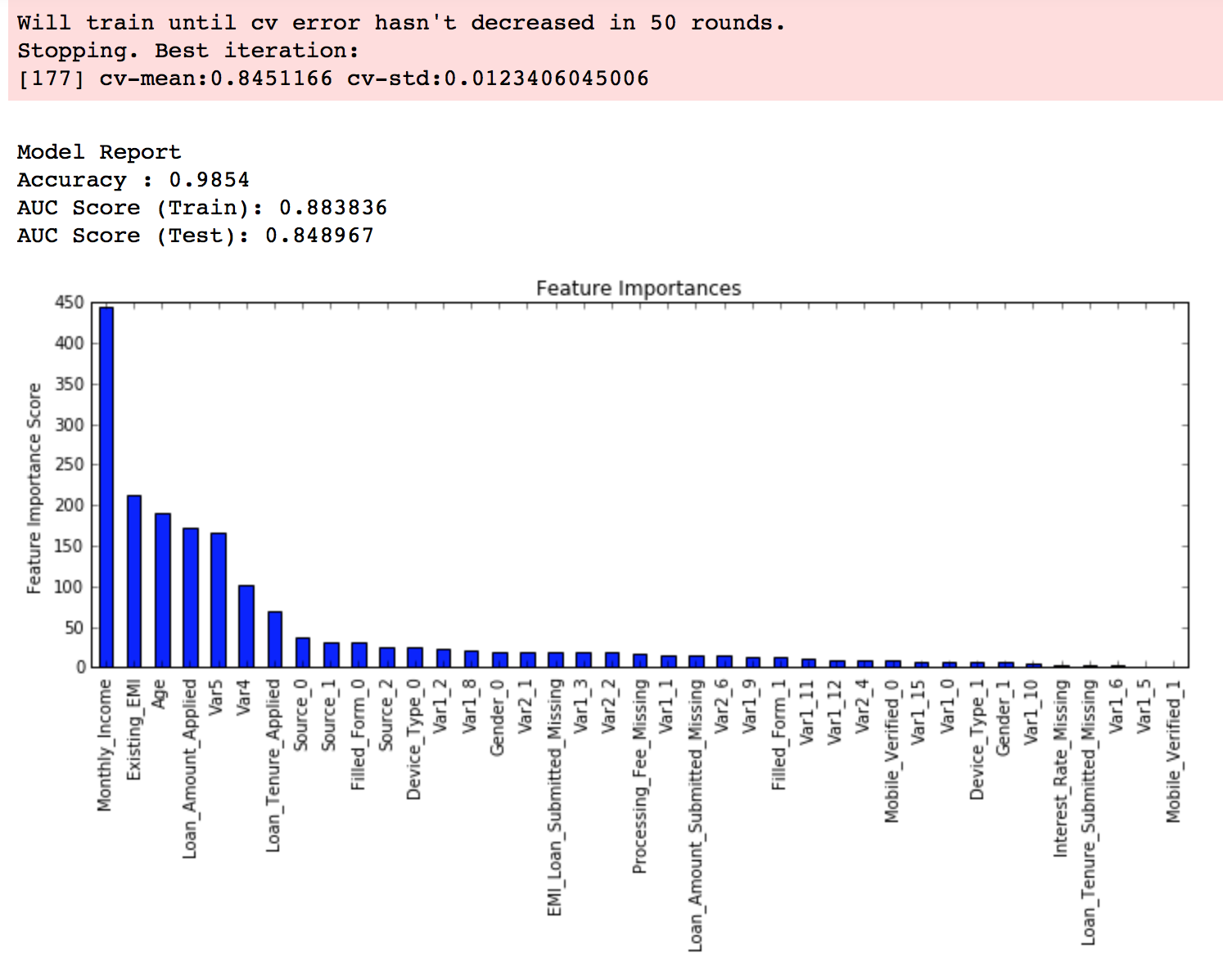
def modelfit(alg, dtrain, predictors,useTrainCV=True, cv_folds=5, early_stopping_rounds=50):
    
    if useTrainCV:
        xgb_param = alg.get_xgb_params()
        xgtrain = xgb.DMatrix(dtrain[predictors].values, label=dtrain[target].values)
        cvresult = xgb.cv(xgb_param, xgtrain, num_boost_round=alg.get_params()['n_estimators'], nfold=cv_folds,
            metrics='auc', early_stopping_rounds=early_stopping_rounds, show_progress=False)
        alg.set_params(n_estimators=cvresult.shape[0])
    
    #Fit the algorithm on the data
    alg.fit(dtrain[predictors], dtrain['Disbursed'],eval_metric='auc')
        
    #Predict training set:
    dtrain_predictions = alg.predict(dtrain[predictors])
    dtrain_predprob = alg.predict_proba(dtrain[predictors])[:,1]
        
    #Print model report:
    print "\nModel Report"
    print "Accuracy : %.4g" % metrics.accuracy_score(dtrain['Disbursed'].values, dtrain_predictions)
    print "AUC Score (Train): %f" % metrics.roc_auc_score(dtrain['Disbursed'], dtrain_predprob)
                    
    feat_imp = pd.Series(alg.booster().get_fscore()).sort_values(ascending=False)
    feat_imp.plot(kind='bar', title='Feature Importances')
    plt.ylabel('Feature Importance Score')

This code is slightly different from what I used for GBM. The focus of this article is to cover the concepts and not coding. Please feel free to drop a note in the comments if you find any challenges in understanding any part of it. Note that xgboost’s sklearn wrapper doesn’t have a “feature_importances” metric but a get_fscore() function which does the same job.

 

General Approach for Parameter Tuning

We will use an approach similar to that of GBM here. The various steps to be performed are:

1. Choose a relatively high learning rate. Generally a learning rate of 0.1 works but somewhere between 0.05 to 0.3 should work for different problems. Determine the optimum number of trees for this learning rate. XGBoost has a very useful function called as “cv” which performs cross-validation at each boosting iteration and thus returns the optimum number of trees required.
2. Tune tree-specific parameters ( max_depth, min_child_weight, gamma, subsample, colsample_bytree) for decided learning rate and number of trees. Note that we can choose different parameters to define a tree and I’ll take up an example here.
3. Tune regularization parameters (lambda, alpha) for xgboost which can help reduce model complexity and enhance performance.
4. Lower the learning rate and decide the optimal parameters .

Let us look at a more detailed step by step approach.

 

Step 1: Fix learning rate and number of estimators for tuning tree-based parameters

In order to decide on boosting parameters, we need to set some initial values of other parameters. Lets take the following values:

1. max_depth = 5 : This should be between 3-10. I’ve started with 5 but you can choose a different number as well. 4-6 can be good starting points.
2. min_child_weight = 1 : A smaller value is chosen because it is a highly imbalanced class problem and leaf nodes can have smaller size groups.
3. gamma = 0 : A smaller value like 0.1-0.2 can also be chosen for starting. This will anyways be tuned later.
4. subsample, colsample_bytree = 0.8 : This is a commonly used used start value. Typical values range between 0.5-0.9.
5. scale_pos_weight = 1: Because of high class imbalance.

Please note that all the above are just initial estimates and will be tuned later. Lets take the default learning rate of 0.1 here and check the optimum number of trees using cv function of xgboost. The function defined above will do it for us.

#Choose all predictors except target & IDcols
predictors = [x for x in train.columns if x not in [target, IDcol]]
xgb1 = XGBClassifier(
 learning_rate =0.1,
 n_estimators=1000,
 max_depth=5,
 min_child_weight=1,
 gamma=0,
 subsample=0.8,
 colsample_bytree=0.8,
 objective= 'binary:logistic',
 nthread=4,
 scale_pos_weight=1,
 seed=27)
modelfit(xgb1, train, predictors)

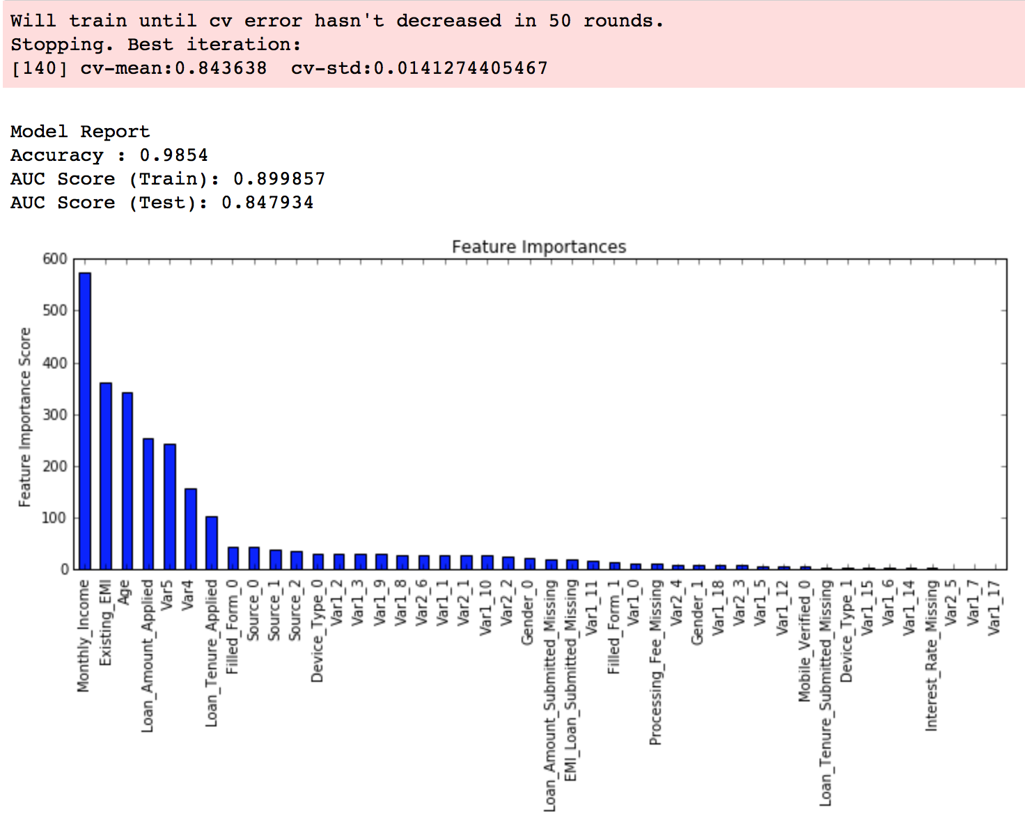
As you can see that here we got 140 as the optimal estimators for 0.1 learning rate. Note that this value might be too high for you depending on the power of your system. In that case you can increase the learning rate and re-run the command to get the reduced number of estimators.

Note: You will see the test AUC as “AUC Score (Test)” in the outputs here. But this would not appear if you try to run the command on your system as the data is not made public. It’s provided here just for reference. The part of the code which generates this output has been removed here.

 

Step 2: Tune max_depth and min_child_weight

We tune these first as they will have the highest impact on model outcome. To start with, let’s set wider ranges and then we will perform another iteration for smaller ranges.

Important Note: I’ll be doing some heavy-duty grid searched in this section which can take 15-30 mins or even more time to run depending on your system. You can vary the number of values you are testing based on what your system can handle.

param_test1 = {
 'max_depth':range(3,10,2),
 'min_child_weight':range(1,6,2)
}
gsearch1 = GridSearchCV(estimator = XGBClassifier( learning_rate =0.1, n_estimators=140, max_depth=5,
 min_child_weight=1, gamma=0, subsample=0.8, colsample_bytree=0.8,
 objective= 'binary:logistic', nthread=4, scale_pos_weight=1, seed=27), 
 param_grid = param_test1, scoring='roc_auc',n_jobs=4,iid=False, cv=5)
gsearch1.fit(train[predictors],train[target])
gsearch1.grid_scores_, gsearch1.best_params_, gsearch1.best_score_

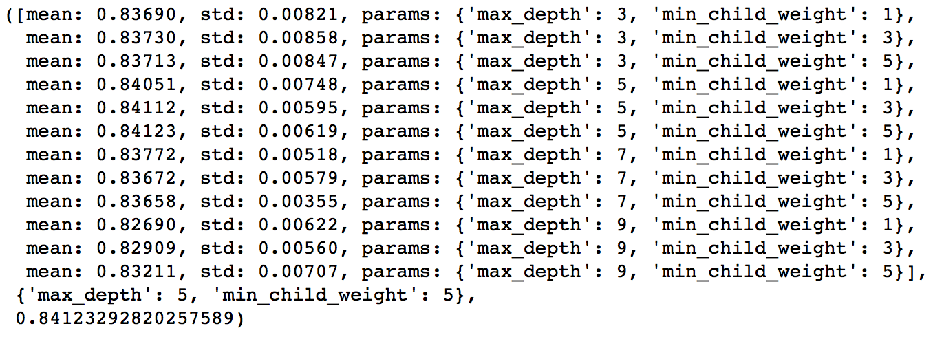
Here, we have run 12 combinations with wider intervals between values. The ideal values are 5 for max_depth and 5 for min_child_weight. Lets go one step deeper and look for optimum values. We’ll search for values 1 above and below the optimum values because we took an interval of two.

param_test2 = {
 'max_depth':[4,5,6],
 'min_child_weight':[4,5,6]
}
gsearch2 = GridSearchCV(estimator = XGBClassifier( learning_rate=0.1, n_estimators=140, max_depth=5,
 min_child_weight=2, gamma=0, subsample=0.8, colsample_bytree=0.8,
 objective= 'binary:logistic', nthread=4, scale_pos_weight=1,seed=27), 
 param_grid = param_test2, scoring='roc_auc',n_jobs=4,iid=False, cv=5)
gsearch2.fit(train[predictors],train[target])
gsearch2.grid_scores_, gsearch2.best_params_, gsearch2.best_score_

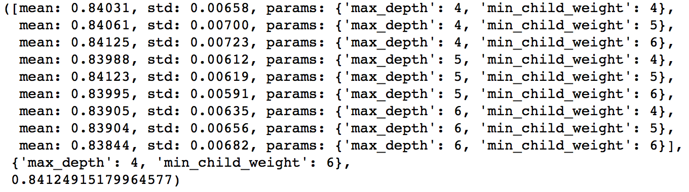
Here, we get the optimum values as 4 for max_depth and 6 for min_child_weight. Also, we can see the CV score increasing slightly. Note that as the model performance increases, it becomes exponentially difficult to achieve even marginal gains in performance. You would have noticed that here we got 6 as optimum value for min_child_weight but we haven’t tried values more than 6. We can do that as follow:.

param_test2b = {
 'min_child_weight':[6,8,10,12]
}
gsearch2b = GridSearchCV(estimator = XGBClassifier( learning_rate=0.1, n_estimators=140, max_depth=4,
 min_child_weight=2, gamma=0, subsample=0.8, colsample_bytree=0.8,
 objective= 'binary:logistic', nthread=4, scale_pos_weight=1,seed=27), 
 param_grid = param_test2b, scoring='roc_auc',n_jobs=4,iid=False, cv=5)
gsearch2b.fit(train[predictors],train[target])

modelfit(gsearch3.best_estimator_, train, predictors)
gsearch2b.grid_scores_, gsearch2b.best_params_, gsearch2b.best_score_

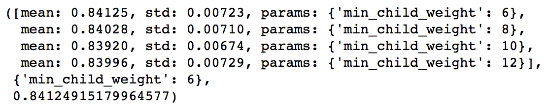
We see 6 as the optimal value.

 

Step 3: Tune gamma

Now lets tune gamma value using the parameters already tuned above. Gamma can take various values but I’ll check for 5 values here. You can go into more precise values as.

param_test3 = {
 'gamma':[i/10.0 for i in range(0,5)]
}
gsearch3 = GridSearchCV(estimator = XGBClassifier( learning_rate =0.1, n_estimators=140, max_depth=4,
 min_child_weight=6, gamma=0, subsample=0.8, colsample_bytree=0.8,
 objective= 'binary:logistic', nthread=4, scale_pos_weight=1,seed=27), 
 param_grid = param_test3, scoring='roc_auc',n_jobs=4,iid=False, cv=5)
gsearch3.fit(train[predictors],train[target])
gsearch3.grid_scores_, gsearch3.best_params_, gsearch3.best_score_

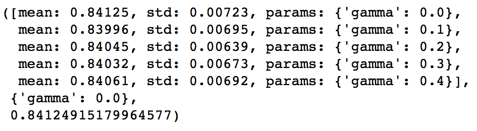
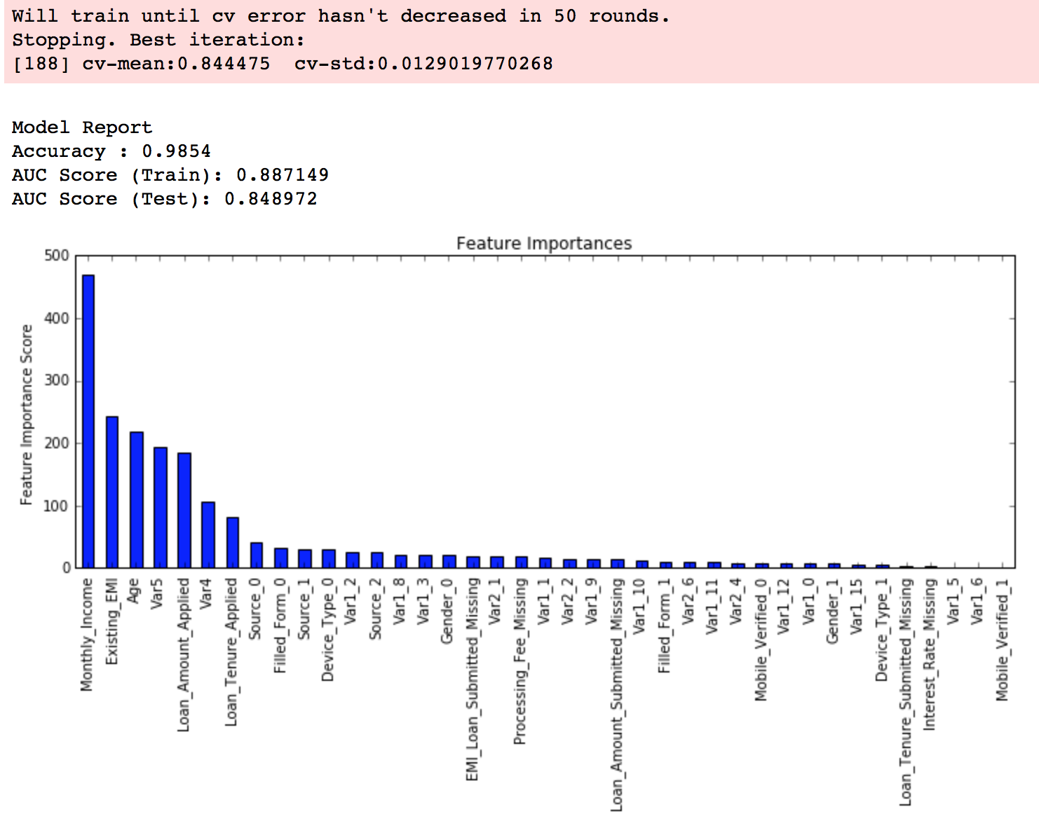
This shows that our original value of gamma, i.e. 0 is the optimum one. Before proceeding, a good idea would be to re-calibrate the number of boosting rounds for the updated parameters.

xgb2 = XGBClassifier(
 learning_rate =0.1,
 n_estimators=1000,
 max_depth=4,
 min_child_weight=6,
 gamma=0,
 subsample=0.8,
 colsample_bytree=0.8,
 objective= 'binary:logistic',
 nthread=4,
 scale_pos_weight=1,
 seed=27)
modelfit(xgb2, train, predictors)

Here, we can see the improvement in score. So the final parameters are:

• max_depth: 4
• min_child_weight: 6
• gamma: 0

 

Step 4: Tune subsample and colsample_bytree

The next step would be try different subsample and colsample_bytree values. Lets do this in 2 stages as well and take values 0.6,0.7,0.8,0.9 for both to start with.

param_test4 = {
 'subsample':[i/10.0 for i in range(6,10)],
 'colsample_bytree':[i/10.0 for i in range(6,10)]
}
gsearch4 = GridSearchCV(estimator = XGBClassifier( learning_rate =0.1, n_estimators=177, max_depth=4,
 min_child_weight=6, gamma=0, subsample=0.8, colsample_bytree=0.8,
 objective= 'binary:logistic', nthread=4, scale_pos_weight=1,seed=27), 
 param_grid = param_test4, scoring='roc_auc',n_jobs=4,iid=False, cv=5)
gsearch4.fit(train[predictors],train[target])
gsearch4.grid_scores_, gsearch4.best_params_, gsearch4.best_score_

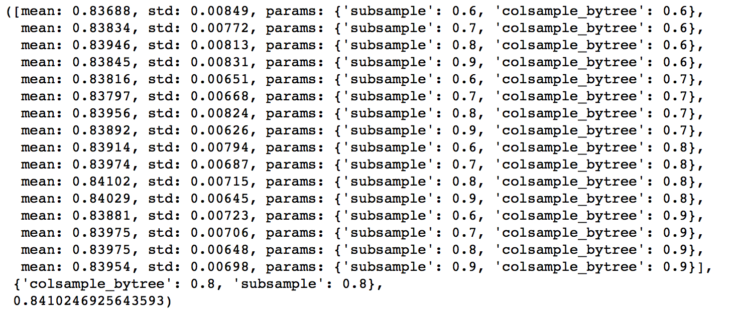
Here, we found 0.8 as the optimum value for both subsample and colsample_bytree. Now we should try values in 0.05 interval around these.

param_test5 = {
 'subsample':[i/100.0 for i in range(75,90,5)],
 'colsample_bytree':[i/100.0 for i in range(75,90,5)]
}
gsearch5 = GridSearchCV(estimator = XGBClassifier( learning_rate =0.1, n_estimators=177, max_depth=4,
 min_child_weight=6, gamma=0, subsample=0.8, colsample_bytree=0.8,
 objective= 'binary:logistic', nthread=4, scale_pos_weight=1,seed=27), 
 param_grid = param_test5, scoring='roc_auc',n_jobs=4,iid=False, cv=5)
gsearch5.fit(train[predictors],train[target])

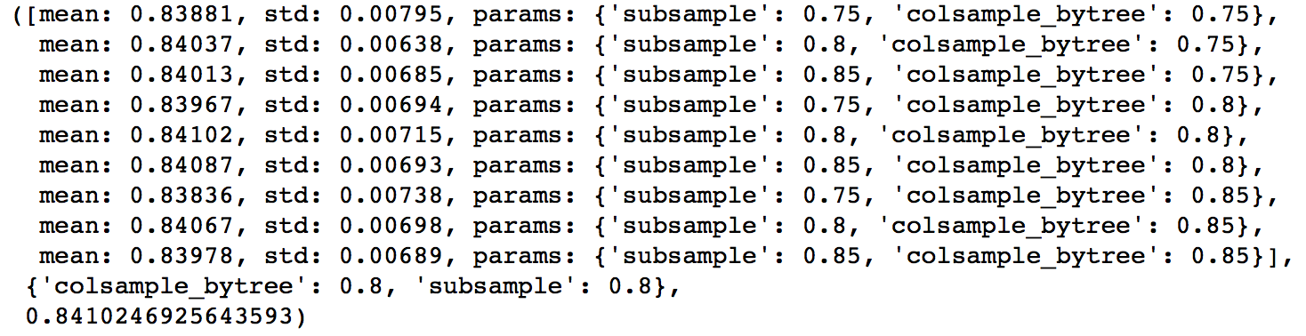
Again we got the same values as before. Thus the optimum values are:

• subsample: 0.8
• colsample_bytree: 0.8

 

Step 5: Tuning Regularization Parameters

Next step is to apply regularization to reduce overfitting. Though many people don’t use this parameters much as gamma provides a substantial way of controlling complexity. But we should always try it. I’ll tune ‘reg_alpha’ value here and leave it upto you to try different values of ‘reg_lambda’.

param_test6 = {
 'reg_alpha':[1e-5, 1e-2, 0.1, 1, 100]
}
gsearch6 = GridSearchCV(estimator = XGBClassifier( learning_rate =0.1, n_estimators=177, max_depth=4,
 min_child_weight=6, gamma=0.1, subsample=0.8, colsample_bytree=0.8,
 objective= 'binary:logistic', nthread=4, scale_pos_weight=1,seed=27), 
 param_grid = param_test6, scoring='roc_auc',n_jobs=4,iid=False, cv=5)
gsearch6.fit(train[predictors],train[target])
gsearch6.grid_scores_, gsearch6.best_params_, gsearch6.best_score_

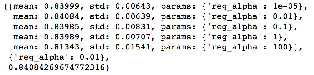
We can see that the CV score is less than the previous case. But the values tried are very widespread, we should try values closer to the optimum here (0.01) to see if we get something better.

param_test7 = {
 'reg_alpha':[0, 0.001, 0.005, 0.01, 0.05]
}
gsearch7 = GridSearchCV(estimator = XGBClassifier( learning_rate =0.1, n_estimators=177, max_depth=4,
 min_child_weight=6, gamma=0.1, subsample=0.8, colsample_bytree=0.8,
 objective= 'binary:logistic', nthread=4, scale_pos_weight=1,seed=27), 
 param_grid = param_test7, scoring='roc_auc',n_jobs=4,iid=False, cv=5)
gsearch7.fit(train[predictors],train[target])
gsearch7.grid_scores_, gsearch7.best_params_, gsearch7.best_score_

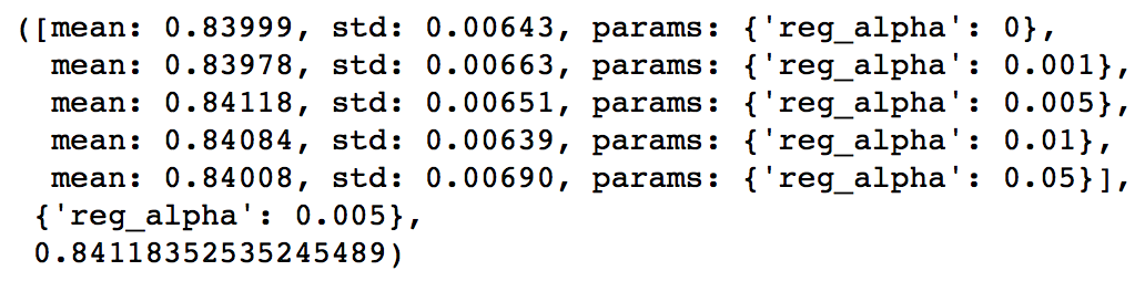
You can see that we got a better CV. Now we can apply this regularization in the model and look at the impact:

xgb3 = XGBClassifier(
 learning_rate =0.1,
 n_estimators=1000,
 max_depth=4,
 min_child_weight=6,
 gamma=0,
 subsample=0.8,
 colsample_bytree=0.8,
 reg_alpha=0.005,
 objective= 'binary:logistic',
 nthread=4,
 scale_pos_weight=1,
 seed=27)
modelfit(xgb3, train, predictors)

Again we can see slight improvement in the score.

Step 6: Reducing Learning Rate

Lastly, we should lower the learning rate and add more trees. Lets use the cv function of XGBoost to do the job again.

xgb4 = XGBClassifier(
 learning_rate =0.01,
 n_estimators=5000,
 max_depth=4,
 min_child_weight=6,
 gamma=0,
 subsample=0.8,
 colsample_bytree=0.8,
 reg_alpha=0.005,
 objective= 'binary:logistic',
 nthread=4,
 scale_pos_weight=1,
 seed=27)
modelfit(xgb4, train, predictors)

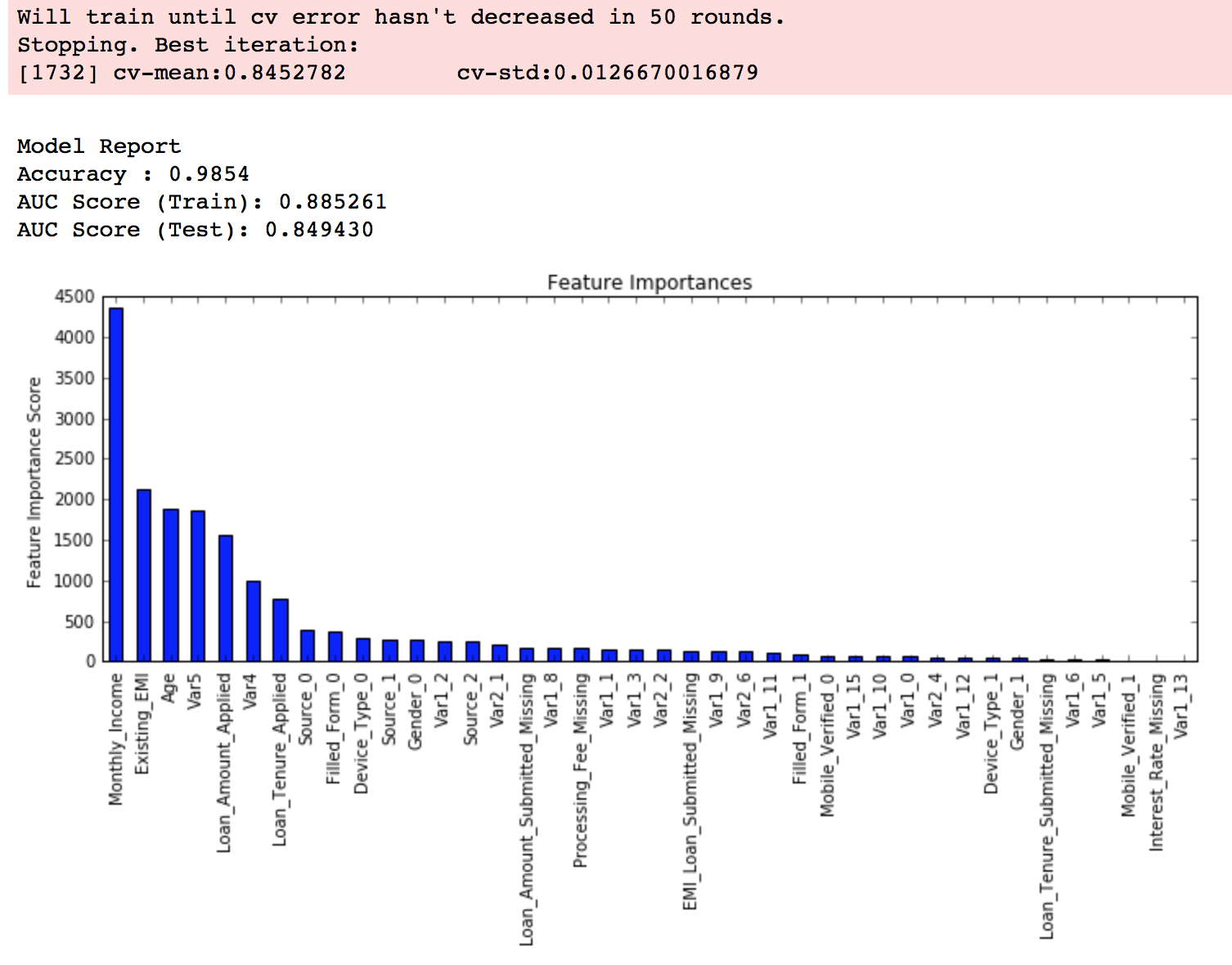
Now we can see a significant boost in performance and the effect of parameter tuning is clearer.

As we come to the end, I would like to share 2 key thoughts:

1. It is difficult to get a very big leap in performance by just using parameter tuning or slightly better models. The max score for GBM was 0.8487 while XGBoost gave 0.8494. This is a decent improvement but not something very substantial.
2. A significant jump can be obtained by other methods like feature engineering, creating ensemble of models, stacking, etc

You can also download the iPython notebook with all these model codes from my GitHub account. For codes in R, you can refer to this article.

 

End Notes

This article was based on developing a XGBoost model end-to-end. We started with discussing why XGBoost has superior performance over GBM which was followed by detailed discussion on thevarious parameters involved. We also defined a generic function which you can re-use for making models.

Finally, we discussed the general approach towards tackling a problem with XGBoost and also worked out the AV Data Hackathon 3.x problem through that approach.

I hope you found this useful and now you feel more confident to apply XGBoost in solving a data science problem. You can try this out in out upcoming hackathons.

Did you like this article? Would you like to share some other hacks which you implement while making XGBoost models? Please feel free to drop a note in the comments below and I’ll be glad to discuss.

You want to apply your analytical skills and test your potential? Then participate in our Hackathons and compete with Top Data Scientists from all over the world.

AI²: Training a big data machine to defend Veeramachaneni et al.IEEE International conference on Big Data Security, 2016

Will machines take over? The lesson of today’s paper is that we’re better off together. Combining AI with HI (human intelligence, I felt like we deserved an acronym of our own ) yields much better results than a system that uses only unsupervised learning. The context is information security, scanning millions of log entries per day to detect suspicious activity and prevent attacks. Examples of attacks include account takeovers, new account fraud (opening a new account using stolen credit card information), and terms of service abuse (e.g. abusing promotional codes, or manipulating cookies for advantage).

A typical attack has a behavioral signature, which comprises the series of steps involved in commiting it. The information necessary to quantify these signatures is buried deep in the raw data, and is often delivered as logs.

The usual problem with such outlier/anomaly detection systems is that they trigger lots of false positive alarms, that take substantial time and effort to investigate. After the system has ‘cried wolf’ enough times they can become distrusted and of limited use. AI² combines the experience and intuition of analysts with machine learning techniques. An ensemble of unsupervised learning models generates a set of k events to be analysed per day (where the daily budget k of events that can be analysed is a configurable parameter). The human judgements on these k events are used to train a supervised model, the results of which are combined with the unsupervised ensemble results to refine the k events to be presented to the analyst on the next day. And so it goes on.

The end result looks a bit like this:

With a daily investigation budget (k) of 200 events, AI² detects 86.8% of attacks with a false positive rate of 4.4%. Using only unsupervised learning, on 7.9% of attacks are detected. If the investigation budget is upped to 1000 events/day, unsupervised learning can detect 73.7% of attacks with a false positive rate of 22%. At this level, the unsupervised system is generating 5x the false positives of AI², and still not detecting as many attacks.

Detecting attacks is a true ‘needle-in-a-haystack’ problem as the following table shows:

Entities in the above refers to the number of unique IP addresses, users, sessions etc. anaysed on a daily basis. The very small relative number of true attacks results in extreme class imbalance when trying to learn a supervised model.

AI² tracks activity based on ingested log records and aggregates activities over intervals of time (for example,counters, indicators – did this happen in the window at all? – elapsed time between events, number of unique values and so on). These features are passed into an ensemble of three unsupervised outlier detection models:

• A Principle Component Analysis (PCA) based model. The basic idea is to use PCA to determine the most significant features (those that explain most of the variance in the data). Given an input take its PCA projection, and then from the projection, reconstruct the original variables. The reconstruction error will be small for the majority of examples, but will remain high for outliers.
• A Replicator Neural Network (not to be confused with a RecurrentNeural Network – both get abbreviated to RNN). This works on a very similar principal. The input and output layers have the same number of nodes, and intermediate layers have fewer nodes. The goal is to train the network to recreate the input at the output layer – which means it must learn an efficient compressed representation in the lower-dimensional hidden layers. Once the RNN has been trained, the reconstruction error can be used as the outlier score.

• The third unsupervised model uses copula functions to build a joint probability function that can be used to detect rare events.

A copula framework provides a means of inference after modeling a multivariate joint probability distribution from training data. Because copula frameworks are less well known than other forms of estimation, we will now briefly review copula theory…

(If you’re interested in that review, and how copula functions are used to form a multivariate density function, see section 6.3 in the paper).

The scores from each of the models are translated into probabilities using a Weibull distribution, “which is flexible and can model a wide variety of shapes.” This translation means that we can compare like-with-like when combining the results from the three models. Here’s an example of the combination process using one-day’s worth of data:

The whole AI² system cycles through training, deployment, and feedback collection/model updating phases on a daily basis. The system trains unsupervised and supervised models based on all the available data, applies those models to the incoming data, identifies k entities as extreme events or attacks, and brings these to the analyst’s attention. The analysts deductions are used to build a new predictive model for the next day.

This combined approach makes effective use of the limited available analyst bandwidth, can overcome some of the weaknesses of pure unsupervised learning, and actively adapts and synthesizes new models.

This setup captures the cascading effect of the human-machine interaction: the more attacks the predictive system detects, the more feeback it will receive from the analysts; this feedback, in turn, will improve the accuracy of future predictions.

---

We often encounter confusion and hype surrounding the terminology of Artificial Intelligence. In this post, it is hoped that the security practitioner can have a quick reference guide for some of the more important and common terms.

Note that this is a limited set. We discovered that, once you start defining these terms, the terms themselves introduce new terms that require definition. We had to draw the line somewhere…

• Artificial Intelligence – “The goal of work in Artificial Intelligence is to build machines that perform tasks that normally require human intelligence.” This quote from Nils Nilsson is an excellent definition, but it is not the only one. There are many definitions of Artificial Intelligence here and here.
• Algorithms – are a self-contained step-by-step sets of operations to be performed. Algorithms perform calculation, data processing, and/or automated reasoning tasks. Among other things, Algorithms can be used to train Machine Learning models.
• Machine Learning – A discipline or subfield of Artificial Intelligence. Paraphrasing the definition by Tom Mitchell, ML is the study of computer algorithms that learn from experience to perform a set of predefined tasks.
• Machine Learning Models – The output of a machine learning algorithm. There are two types of machine learning models, those generated by Supervised algorithms and Unsupervised algorithms. See below.
• The difference between “algorithms” and “models”: this is a common question and still quite difficult to answer. In the context of Artificial Intelligence, we can say that learning algorithms generate models. The learning algorithms are either Supervised or Unsupervised.N.B. People often use “models” and “algorithms” interchangeably which is a common source of confusion. To the layman, think that algorithms are like programs and the models are the output of the program.  
• Unsupervised Learning (algorithm) – a family of machine learning algorithms that learn without labels (labels defined below). The output of Unsupervised Learning algorithms are models that capture the structure of the data, can identify groups, or find statistical outliers. For example, Unsupervised Learning models can show you behaviors that are unlike other behaviors in a corpus of data.
• Supervised Learning (algorithm) – a family of machine learning algorithms that learn from labeled data. The output of Supervised Learning algorithms are predictive models that can classify or assign a score to a data pattern. For example, trained Supervised Learning models can classify behaviors patterns into different attack tactics, or can assign a risk score to a behavior. In cyber-security, Supervised Learning models predict what a human would label a given behavior pattern.
• Labeling – is the act of classification or describing something. For PatternEx, the act of labeling is something that a human analyst does every day. He or she marks something as a malicious or benign behavior. The more labels are provided, the more accurate the system becomes.
• Active Learning – Active learning is a machine learning process in which a learning algorithm interactively requests inputs from an external source to improve a model. It is most commonly applied when only unlabeled data is available, the goal is to train Supervised Learning models, and the external source is a human expert that provides labels, and the labeling process is expensive and/or slow. Active learning strategies are also useful when, as in the case of InfoSec, the data changes fast.
• Behavior Vectors – a quantified description of the activity of the modeled entities.
• Entities – a thing with distinct, independent existence against which the behaviors relate. In cyber-security, examples would be users, IP’s, domains, and so on.
• Human-Assisted Artificial Intelligence – the synergy between human intuition and artificial intelligence. Note that the humans assist the AI by providing feedback (e.g. labels) and the trained AI assists the humans by automating and scaling the tasks requiring human intelligence.
• Predictions – are the activity of the system anticipating how an event would be classified by the security analyst.
• Rare Events – very similar to “anomalies” and “outliers,” Rare Events are events that activities seen in log data that are unusual or out of the ordinary but not yet determined to be either malicious or benign.
• Transfer Learning – means you can port knowledge acquired at one environment to another to improve model accuracy. For example, a model trained at company X can be transferred to companies A, B and C, increasing the detection capabilities of the entire group.
• Virtual Analyst – the term that describes the effect of a fully trained AI system. Because a trained AI system greatly scales the analytic capability of the human analyst team, we say it is like expanding your team with “virtual analysts.”

PatternEx Unique Approach

PatternEx comes with many algorithms out-of-the-box that allow it to create predictive models that select what the analyst should review. Humans will always be needed to identify in context what is malicious in a constantly changing sea of events. In this way, Human-Assisted Artificial intelligence systems learn from analysts to identify what events are malicious. This results in greater detection accuracy at scale and reduced mean time to identify an attack.

If you’d like to learn more about how PatternEx is bringing Artificial Intelligence into the domain of Cyber Security click here:  LEARN MORE