Fields Medalist:
Artur Avila

CNRS, France & IMPA, Brazil
[Artur Avila is awarded a Fields Medal] for his profound contributions to dynamical systems theory have changed the face of the field, using the powerful idea of renormalization as a unifying principle.
Avila leads and shapes the field of dynamical systems. With his collaborators, he has made essential progress in many areas, including real and complex one-dimensional dynamics, spectral theory of the one-frequency Schródinger operator, flat billiards and partially hyperbolic dynamics.
Avila’s work on real one-dimensional dynamics brought completion to the subject, with full understanding of the probabilistic point of view, accompanied by a complete renormalization theory. His work in complex dynamics led to a thorough understanding of the fractal geometry of Feigenbaum Julia sets.
In the spectral theory of one-frequency difference Schródinger operators, Avila came up with a global de- scription of the phase transitions between discrete and absolutely continuous spectra, establishing surprising stratified analyticity of the Lyapunov exponent.
In the theory of flat billiards, Avila proved several long-standing conjectures on the ergodic behavior of interval-exchange maps. He made deep advances in our understanding of the stable ergodicity of typical partially hyperbolic systems.
Avila’s collaborative approach is an inspiration for a new generation of mathematicians.
Manjul Bhargava

Princeton University, USA
[Manjul Bhargava is awarded a Fields Medal] for developing powerful new methods in the geometry of numbers and applied them to count rings of small rank and to bound the average rank of elliptic curves.
Bhargava’s thesis provided a reformulation of Gauss’s law for the composition of two binary quadratic forms. He showed that the orbits of the group SL(2, Z)3 on the tensor product of three copies of the standard integral representation correspond to quadratic rings (rings of rank 2 over Z) together with three ideal classes whose product is trivial. This recovers Gauss’s composition law in an original and computationally effective manner. He then studied orbits in more complicated integral representations, which correspond to cubic, quartic, and quintic rings, and counted the number of such rings with bounded discriminant.
Bhargava next turned to the study of representations with a polynomial ring of invariants. The simplest such representation is given by the action of PGL(2, Z) on the space of binary quartic forms. This has two independent invariants, which are related to the moduli of elliptic curves. Together with his student Arul Shankar, Bhargava used delicate estimates on the number of integral orbits of bounded height to bound the average rank of elliptic curves. Generalizing these methods to curves of higher genus, he recently showed that most hyperelliptic curves of genus at least two have no rational points.
Bhargava’s work is based both on a deep understanding of the representations of arithmetic groups and a unique blend of algebraic and analytic expertise.
Martin Hairer
University of Warwick, UK
[Martin Hairer is awarded a Fields Medal] for his outstanding contributions to the theory of stochastic partial differential equations, and in particular created a theory of regularity structures for such equations.
A mathematical problem that is important throughout science is to understand the influence of noise on differential equations, and on the long time behavior of the solutions. This problem was solved for ordinary differential equations by Itó in the 1940s. For partial differential equations, a comprehensive theory has proved to be more elusive, and only particular cases (linear equations, tame nonlinearities, etc.) had been treated satisfactorily.
Hairer’s work addresses two central aspects of the theory. Together with Mattingly he employed the Malliavin calculus along with new methods to establish the ergodicity of the two-dimensional stochastic Navier-Stokes equation.
Building on the rough-path approach of Lyons for stochastic ordinary differential equations, Hairer then created an abstract theory of regularity structures for stochastic partial differential equations (SPDEs). This allows Taylor-like expansions around any point in space and time. The new theory allowed him to construct systematically solutions to singular non-linear SPDEs as fixed points of a renormalization procedure.
Hairer was thus able to give, for the first time, a rigorous intrinsic meaning to many SPDEs arising in physics.
Maryam Mirzakhani

Stanford University, USA
[Maryam Mirzakhani is awarded the Fields Medal] for her outstanding contributions to the dynamics and geometry of Riemann surfaces and their moduli spaces.
Maryam Mirzakhani has made stunning advances in the theory of Riemann surfaces and their moduli spaces, and led the way to new frontiers in this area. Her insights have integrated methods from diverse fields, such as algebraic geometry, topology and probability theory.
In hyperbolic geometry, Mirzakhani established asymptotic formulas and statistics for the number of simple closed geodesics on a Riemann surface of genus g. She next used these results to give a new and completely unexpected proof of Witten’s conjecture, a formula for characteristic classes for the moduli spaces of Riemann surfaces with marked points.
In dynamics, she found a remarkable new construction that bridges the holomorphic and symplectic aspects of moduli space, and used it to show that Thurston’s earthquake flow is ergodic and mixing.
Most recently, in the complex realm, Mirzakhani and her coworkers produced the long sought-after proof of the conjecture that – while the closure of a real geodesic in moduli space can be a fractal cobweb, defying classification – the closure of a complex geodesic is always an algebraic subvariety.
Her work has revealed that the rigidity theory of homogeneous spaces (developed by Margulis, Ratner and others) has a definite resonance in the highly inhomogeneous, but equally fundamental realm of moduli spaces, where many developments are still unfolding
Nevanlinna Prize Winner:
Subhash Khot

New York University, USA
[Subhash Khot is awarded the Nevanlinna Prize] for his prescient definition of the “Unique Games” problem, and his leadership in the effort to understand its complexity and its pivotal role in the study of efficient approximation of optimization problems, have produced breakthroughs in algorithmic design and approximation hardness, and new exciting interactions between computational complexity, analysis and geometry.
Subhash Khot defined the “Unique Games” in 2002 , and subsequently led the effort to understand its complexity and its pivotal role in the study of optimization problems. Khot and his collaborators demonstrated that the hardness of Unique Games implies a precise characterization of the best approximation factors achievable for a variety of NP-hard optimization problems. This discovery turned the Unique Games problem into a major open problem of the theory of computation.
The ongoing quest to study its complexity has had unexpected benefits. First, the reductions used in the above results identified new problems in analysis and geometry, invigorating analysis of Boolean functions, a field at the interface of mathematics and computer science. This led to new central limit theorems, invariance principles, isoperimetric inequalities, and inverse theorems, impacting research in computational complexity, pseudorandomness, learning and combinatorics. Second, Khot and his collaborators used intuitions stemming from their study of Unique Games to yield new lower bounds on the distortion incurred when embedding one metric space into another, as well as constructions of hard families of instances for common linear and semi- definite programming algorithms. This has inspired new work in algorithm design extending these methods, greatly enriching the theory of algorithms and its applications.
Gauss Prize Winner:
Stanley Osher

University of Califonia, USA
[Stanley Osher is awarded the Gauss Prize] for his influential contributions to several fields in applied mathematics, and his far-ranging inventions have changed our conception of physical, perceptual, and mathematical concepts, giving us new tools to apprehend the world.
1. Stanley Osher has made influential contributions in a broad variety of fields in applied mathematics. These include high resolution shock capturing methods for hyperbolic equations, level set methods, PDE based methods in computer vision and image processing, and optimization. His numerical analysis contributions, including the Engquist-Osher scheme, TVD schemes, entropy conditions, ENO and WENO schemes and numerical schemes for Hamilton-Jacobi type equations have revolutionized the field. His level set contribu- tions include new level set calculus, novel numerical techniques, fluids and materials modeling, variational approaches, high codimension motion analysis, geometric optics, and the computation of discontinuous so- lutions to Hamilton-Jacobi equations; level set methods have been extremely influential in computer vision, image processing, and computer graphics. In addition, such new methods have motivated some of the most fundamental studies in the theory of PDEs in recent years, completing the picture of applied mathematics inspiring pure mathematics.
2. Stanley Osher has unique mentoring qualities: he has influenced the education of generations of outstanding applied mathematicians, and thanks to his entrepreneurship he has successfully brought his mathematics to industry.
Trained as an applied mathematician and an applied mathematician all his life, Osher continues to surprise the mathematical and numerical community with the invention of simple and clever schemes and formulas. His far-ranging inventions have changed our conception of physical, perceptual, and mathematical concepts, and have given us new tools to apprehend the world.
Chern Medalist:
Phillip Griffiths

Institute for Advanced Study, USA
[Phillip Griths is awarded the 2014 Chern Medal] for his groundbreaking and transformative development of transcendental methods in complex geometry, particularly his seminal work in Hodge theory and periods of algebraic varieties.
Phillip Griffiths’s ongoing work in algebraic geometry, differential geometry, and differential equations has stimulated a wide range of advances in mathematics over the past 50 years and continues to influence and inspire an enormous body of research activity today.
He has brought to bear both classical techniques and strikingly original ideas on a variety of problems in real and complex geometry and laid out a program of applications to period mappings and domains, algebraic cycles, Nevanlinna theory, Brill-Noether theory, and topology of K¨ahler manifolds.
A characteristic of Griffithss work is that, while it often has a specific problem in view, it has served in multiple instances to open up an entire area to research.
Early on, he made connections between deformation theory and Hodge theory through infinitesimal methods, which led to his discovery of what are now known as the Griffiths infinitesimal period relations. These methods provided the motivation for the Griffiths intermediate Jacobian, which solved the problem of showing algebraic equivalence and homological equivalence of algebraic cycles are distinct. His work with C.H. Clemens on the non-rationality of the cubic threefold became a model for many further applications of transcendental methods to the study of algebraic varieties.
His wide-ranging investigations brought many new techniques to bear on these problems and led to insights and progress in many other areas of geometry that, at first glance, seem far removed from complex geometry. His related investigations into overdetermined systems of differential equations led a revitalization of this subject in the 1980s in the form of exterior differential systems, and he applied this to deep problems in modern differential geometry: Rigidity of isometric embeddings in the overdetermined case and local existence of smooth solutions in the determined case in dimension 3, drawing on deep results in hyperbolic PDEs(in collaborations with Berger, Bryant and Yang), as well as geometric formulations of integrability in the calculus of variations and in the geometry of Lax pairs and treatises on the geometry of conservation laws and variational problems in elliptic, hyperbolic and parabolic PDEs and exterior differential systems.
All of these areas, and many others in algebraic geometry, including web geometry, integrable systems, and Riemann surfaces, are currently seeing important developments that were stimulated by his work.
His teaching career and research leadership has inspired an astounding number of mathematicians who have gone on to stellar careers, both in mathematics and other disciplines. He has been generous with his time, writing many classic expository papers and books, such as “Principles of Algebraic Geometry”, with Joseph Harris, that have inspired students of the subject since the 1960s.
Griffiths has also extensively supported mathematics at the level of research and education through service on and chairmanship of numerous national and international committees and boards committees and boards. In addition to his research career, he served 8 years as Duke’s Provost and 12 years as the Director of the Institute for Advanced Study, and he currently chairs the Science Initiative Group, which assists the development of mathematical training centers in the developing world.
His legacy of research and service to both the mathematics community and the wider scientific world continues to be an inspiration to mathematicians world-wide, enriching our subject and advancing the discipline in manifold ways.
Leelavati Prize Winner:
Adrián Paenza

University of Buenos Aires, Argentina
[Adrian Paenza is awarded the Leelavati Prize] for his contributions have definitively changed the mind of a whole country about the way it perceives mathematics in daily life. He accomplished this through his books, his TV programs, and his unique gift of enthusiasm and passion in communicating the beauty and joy of mathematics.
Adrián Paenza has been the host of the long-running weekly TV program “Cient´ıficos Industria Argentina” (“Scientists Made in Argentina”), currently in its twelfth consecutive season in an open TV channel. Within a beautiful and attractive interface, each program consists of interviews with mathematicians and scientists of very different disciplines, and ends with a mathematical problem, the solution of which is given in the next program.
He has also been the host of the TV program “Alterados por Pi” (“Altered by Pi”), a weekly half-hour show exclusively dedicated to the popularization of mathematics; this show is recorded in front of a live audience in several public schools around the country.
Since 2005, he has written a weekly column about general science, but mainly about mathematics, on the back page of P´agina 12, one of Argentinas three national newspapers. His articles include historical notes, teasers and even proofs of theorems.
He has written eight books dedicated to the popularization of mathematics: five under the name “Matem´atica
. . . ¿est´as ah´ı?” (“Math . . . are you there?”), published by Siglo XXI Editores, which have sold over a million copies. The first of the series, published in September 2005, headed the lists of best sellers for a record of 73 consecutive weeks, and is now in its 22nd edition. The enormous impact and influence of these books has extended throughout Latin America and Spain; they have also been published in Portugal, Italy, the Czech Republic, and Germany; an upcoming edition has been recently translated also into Chinese.

 which possibly has a finite (or countable) number of discontinuities or points where possibly the derivative does not exist. We assume that there are points
 or
or 
 is
is  , with a bound on the first and the second derivatives. Assume that the interval
 ![[q_{0},q_{k}]](https://s0.wp.com/latex.php?latex=%5Bq_%7B0%7D%2Cq_%7Bk%7D%5D&bg=ffffff&fg=2b2b2b&s=0&c=20201002) ( or
( or ![[q_{0},q_{\infty}]](https://s0.wp.com/latex.php?latex=%5Bq_%7B0%7D%2Cq_%7B%5Cinfty%7D%5D&bg=ffffff&fg=2b2b2b&s=0&c=20201002) ) is positive invariant, so
) is positive invariant, so ![f(x)\in [q_{0},q_{k}]](https://s0.wp.com/latex.php?latex=f%28x%29%5Cin+%5Bq_%7B0%7D%2Cq_%7Bk%7D%5D&bg=ffffff&fg=2b2b2b&s=0&c=20201002) for all
for all ![x\in [q_{0}, q_{k}]](https://s0.wp.com/latex.php?latex=x%5Cin+%5Bq_%7B0%7D%2C+q_%7Bk%7D%5D&bg=ffffff&fg=2b2b2b&s=0&c=20201002) ( or
( or ![f(x)\in [q_{0},q_{\infty}]](https://s0.wp.com/latex.php?latex=f%28x%29%5Cin+%5Bq_%7B0%7D%2Cq_%7B%5Cinfty%7D%5D&bg=ffffff&fg=2b2b2b&s=0&c=20201002) for all
for all ![x\in[q_{0},q_{\infty}]](https://s0.wp.com/latex.php?latex=x%5Cin%5Bq_%7B0%7D%2Cq_%7B%5Cinfty%7D%5D&bg=ffffff&fg=2b2b2b&s=0&c=20201002) ).
). ( or
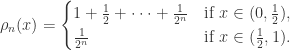
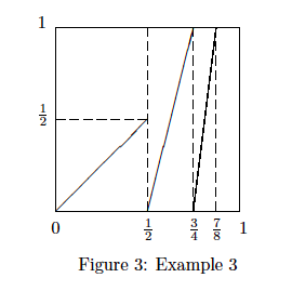
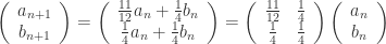
( or  ),assume that we have defined densities up to
  , then define define
  as follows
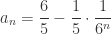
 , which takes one density function to another function, is called the Perron-Frobenius operator. The limit of the first
  density functions converges to a density function
  ,
,
 .
.
 on
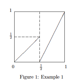
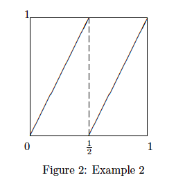
on ![[0,1]](https://s0.wp.com/latex.php?latex=%5B0%2C1%5D&bg=ffffff&fg=2b2b2b&s=0&c=20201002) . From the definition of
. From the definition of  , the slope on
  and
and  are 1 and 2, respectively. If
  , then it has only one pre-image on
  , then it has two pre-images, one is
  in
in  in
in 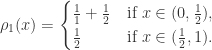


 , then
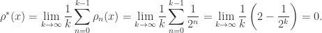


 . By induction,
  on
on  . Therefore,
  on
on 

 . By similar considerations,
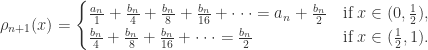

 and
and  for all


 and
and 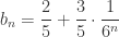 for all
![A=[a_{ij}]](https://s0.wp.com/latex.php?latex=A%3D%5Ba_%7Bij%7D%5D&bg=ffffff&fg=2b2b2b&s=0&c=20201002) be a
be a  matrix. We say
  is non-negative if
  for all
  . Such a matrix is called irreducible if for any pair
  such that
  where
where  is the
  th element of
  . The matrix
  such that no eigenvalue of
  .
. and a non-negative right (column) eigenvector
  .
. ,
,  all
all  ).
). .
. has the largest absolute value in the set of all eigenvalues of
  for all pairs
  . That means
  is a strictly positive
  be a compact interval. A
  map
map  is called Markov if there exists a finite or countable family
  of disjoint open intervals in
  has Lebesgue measure zero and there exist
  and
and  such that for each
  and each interval
  such that
  is contained in one of the intervals
  one has
 , then
  ;
; such that
  for each
  . Usually, we will denote the Lebesgue measure of a Borel set
  .
. be corresponding partition. Then there exists a
  invariant probability measure
  on the Borel sets of
  is uniformly bounded and Holder continuous. Moreover, for each
  one has
  for some
  then
then for every Borel set
  .
. for each interval
  be a sequence of analytic functions on a domain
  which converges uniformly on compact subsets of
  converges uniformly on compact subsets to
  .
. . If
. If  for some
  , then for each
  , such that for all
  ,
,  has the same number of zeros in
  as does
  has no maximum in
  and analytic on the interior of
  is locally bounded on a domain
  , there is a positive number
  and a neighbourhood
  such that
  for all
  and all
  .
. form a locally bounded family in
  . However, the following partial converse does hold.
 is locally bounded and suppose that there is some
  for all
  and
and  .)
.) if, for each
  , there is a
  such that
  ,
,  whenever
  , for every
  if it is continuous (spherically continuous) at each point of
  is normal in
  contains either a subsequence which converges to a limit function
  uniformly on each compact subset of
  on each compact subset.
 of continuous functions converges uniformly on a compact set
  to a limit function
  such that for any
  ,
,  .
. exists for each
  which converges normally to an analytic function
  for each
  . Suppose, however, that
  , as well as a subsequence
  and points
  satisfying
 . Now
. Now  itself has a subsequence which converges uniformly on compact subsets to an analytic function
  , and
, and  from above. However, since
  on
on  and
and  in
in  . Then
  and such that no function of
  at more that
  points. Then
  is the unit disk in the complex plane,
  in
in  . In the domain
  ,
,  is a normal family in
  but not compact.
 analytic in
  . Then
  . Then
  is a uniformly bounded family.
 analytic, univalent in
  . These are the normalised “Schlicht” functions in
  is normal and compact.
 . The point
  between
  and
and  is
is if
if  if
if  . Clearly,
  , and
, and  . The chordal metric and spherical metric are uniformly equivalent and generate the same open sets on the Riemann sphere.
 if, for any
  such that
  implies
  , for all
  contains a subsequence which converges spherically uniformly on compact subsets of
  in which
  or
or  uniformly as
  .
. . Then
  converges spherically on a point set
  is not a pole, the derivative in the spherical metric, called the spherical derivative, is given by
 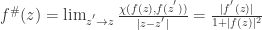 . If
. If  is a pole of
  .
. such that spherical derivative
  that is,
  is locally bounded.
 infinite paraboloid
 hyperbolic paraboloid
 sphere with radius
  and center


 cylinder
 Plane
Plane Parabola
 : 1 question. Especially,
  and
and  (Integration by parts).
 : 1 question, where
  is a positive real number. Especially,
  and
and  .
. and reverse the order of dx and dy).
 and the domain
  plane. If the domain
  , where
  . Pay attention to the orientation of the curve on the boundary, i.e. the right hand rule).
 ).
).


 is called a critical point of f(x), if
 on some interval I, then f(x) is increasing on the interval I. Similarly, if
  on some interval I, then f(x) is decreasing on the interval I.
 is
is  where
where  is the slope of the tangent line.
 is
is  because the Chain Rule of derivatives.
 at the point (16,16).
 at the both sides, we get
 That means the tangent line of the curve at the point (16,16) is y-16=-(x-16). i.e. y=-x+32.
 , then calculating the derivative directly. i.e.
 then (16,16) corresponds to
  From the derivative of the parameter functions, we know
 then
then  and
and  Find dy/dx and express your answer in terms of
 ,
,


 的模型:
的模型: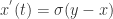


 是这个系统的参数。


 ,然后
,然后
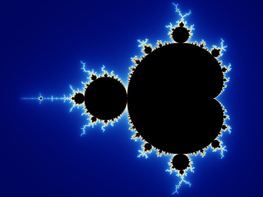
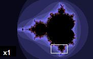
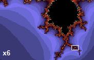
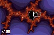
 产生的Mandelbrot集合,还有一些经典的分形结构。比如说Cantor集合。Cantor集合是不断的从一个区间[0,1]取走中间一段获得的集合。首先去掉
 ,剩下
,剩下![[0,\frac{1}{3}] \cup [\frac{2}{3}, 1]](https://s0.wp.com/latex.php?latex=%5B0%2C%5Cfrac%7B1%7D%7B3%7D%5D+%5Ccup+%5B%5Cfrac%7B2%7D%7B3%7D%2C+1%5D&bg=ffffff&fg=2b2b2b&s=0&c=20201002) 。然后把剩下两条线段的中间都去掉,剩下
。然后把剩下两条线段的中间都去掉,剩下![[0,\frac{1}{9}] \cup [\frac{2}{9}, \frac{1}{3}] \cup [\frac{2}{3}, \frac{7}{9}] \cup [\frac{8}{9}, 1]](https://s0.wp.com/latex.php?latex=%5B0%2C%5Cfrac%7B1%7D%7B9%7D%5D+%5Ccup+%5B%5Cfrac%7B2%7D%7B9%7D%2C+%5Cfrac%7B1%7D%7B3%7D%5D+%5Ccup+%5B%5Cfrac%7B2%7D%7B3%7D%2C+%5Cfrac%7B7%7D%7B9%7D%5D+%5Ccup+%5B%5Cfrac%7B8%7D%7B9%7D%2C+1%5D&bg=ffffff&fg=2b2b2b&s=0&c=20201002) 。不停的重复这个过程,最后剩下的集合就是Cantor集合。在数学中,Cantor集合是无穷无尽的,甚至是不可数的,但是却是不占据任何空间的,因为它的长度是零。下图简单的描述了Cantor集合的形成过程。
。不停的重复这个过程,最后剩下的集合就是Cantor集合。在数学中,Cantor集合是无穷无尽的,甚至是不可数的,但是却是不占据任何空间的,因为它的长度是零。下图简单的描述了Cantor集合的形成过程。