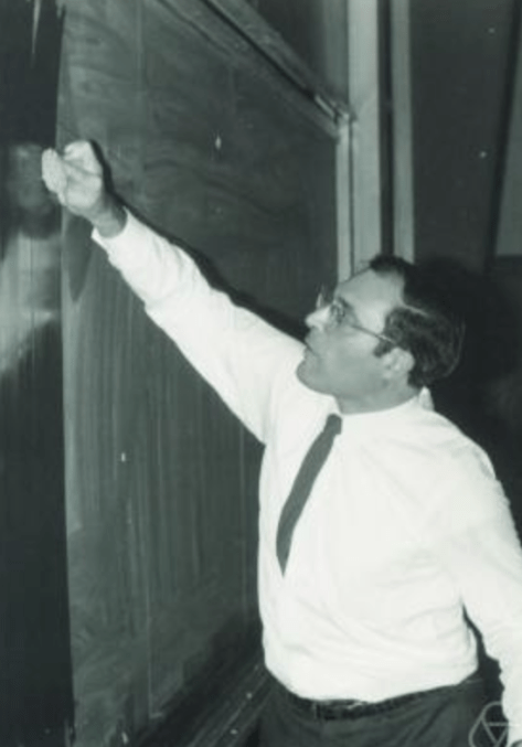
意大利裔的美籍数学家 Gian-Carlo Rota(1932 年 4 月 27 日 – 1999 年 4 月 18 日)是一位杰出的组合学家。他曾是研究泛函分析(Functional Analysis)出身,后来由于个人兴趣的转移,成为了一位研究组合数学(Combinatorial Mathematics)的学者。Rota 的职业生涯大部分都在麻省理工学院(MIT)度过,曾担任 MIT 的数学教授与哲学教授。
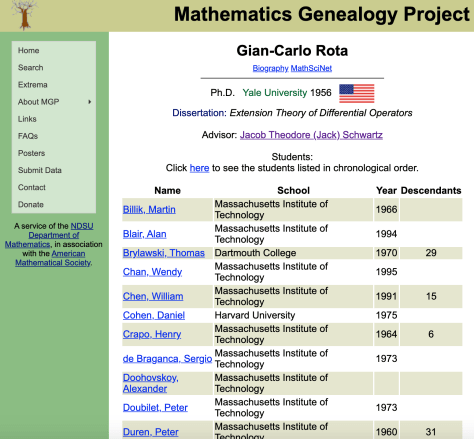
从数学家族谱(Mathematics Genealogy Project)上面可以看到:Gian-Carlo Rota 的导师是 Jacob T. Schwartz,Rota 于 1956 年在耶鲁大学获得数学博士学位,其博士论文的题目是 Extension Theory of Differential Operators。
在 1997 年,Rota 发表了两篇关于人生经验和忠告的文章,分别是 “Ten Lessons I wish I Had Been Taught” 和 “Ten Lessons for the Survival of a Mathematics Department“。下面就来逐一分享这两篇文章中的一些观点。
Ten Lessons I wish I Had Been Taught

讲座(Lecturing)
每次讲座或者分享的时候都有几个需要注意的事情。
(a)每次讲座都应该只有一个重点。(Every lecture should make only one main point.)
Every lecture should state one main point and repeat it over and over, like a theme with variations. An audience is like a herd of cows, moving slowly in the direction they are being driven towards. If we make one point, we have a good chance that the audience will take the right direction; if we make several points, then the cows will scatter all over the field. The audience will lose interest and everyone will go back to the thoughts they interrupted in order to come to our lecture.
(b)不要超时。(Never run overtime.)
Running overtime is the one unforgivable error a lecturer can make. After fifty minutes (one micro-century as von Neumann used to say) everybody’s attention will turn elsewhere even if we are trying to prove the Riemann hypothesis. One minute overtime can destroy the best of lectures.
(c)提及听众的成果。(Relate to your audience.)
As you enter the lecture hall, try to spot someone in the audience with whose work you have some familiarity. Quickly rearrange your presentation so as to manage to mention some of that person’s work. In this way, you will guarantee that at least one person will follow with rapt attention, and you will make a friend to boot.
Everyone in the audience has come to listen to your lecture with the secret hope of hearing their work mentioned.
(d)给听众一些值得回忆的东西。(Give them something to take home.)
Most of the time they admit that they have forgotten the subject of the course and all the mathematics I thought I had taught them. However, they will gladly recall some joke, some anecdote, some quirk, some side remark, or some mistake I made.
板书技巧(Blackboard Technique)
(a)开讲前保持黑板干净(Make sure the blackboard is spotless.)
By starting with a spotless blackboard you will subtly convey the impression that the lecture they are about to hear is equally spotless.
(b)从黑板的左上角开始书写(Start writing on the top left-hand corner.)
What we write on the blackboard should correspond to what we want an attentive listener to take down in his notebook. It is preferable to write slowly and in a large handwriting, with no abbreviations.
When slides are used instead of the blackboard, the speaker should spend some time explaining each slide, preferably by adding sentences that are inessential, repetitive, or superfluous, so as to allow any member of the audience time to copy our slide. We all fall prey to the illusion that a listener will find the time to read the copy of the slides we hand them after the lecture. This is wishful thinking.
多次公布同样的结果(Publish the Same Result Several Times)
The mathematical community is split into small groups, each one with its own customs, notation, and terminology. It may soon be indispensable to present the same result in several versions, each one accessible to a specific group; the price one might have to pay otherwise is to have our work rediscovered by someone who uses a different language and notation and who will rightly claim it as his own.
说明性的工作反而更有可能被记得(You Are More Likely to Be Remembered by Your Expository Work)
When we think of Hilbert, we think of a few of his great theorems, like his basis theorem. But Hilbert’s name is more often remembered for his work in number theory, his Zahlbericht, his book Foundations of Geometry, and for his text on integral equations.
每个数学家只有少数的招数(Every Mathematician Has Only a Few Tricks)
You admire Erdös’s contributions to mathematics as much as I do, and I felt annoyed when the older mathematician flatly and definitively stated that all of Erdös’s work could be “reduced” to a few tricks which Erdös repeatedly relied on in his proofs. What the number theorist did not realize is that other mathematicians, even the very best, also rely on a few tricks which they use over and over. But on reading the proofs of Hilbert’s striking and deep theorems in invariant theory, it was surprising to verify that Hilbert’s proofs relied on the same few tricks. Even Hilbert had only a few tricks!
别害怕犯错(Do Not Worry about Your Mistakes)
There are two kinds of mistakes. There are fatal mistakes that destroy a theory, but there are also contingent ones, which are useful in testing the stability of a theory.
使用费曼的方法(Use the Feynman Method)
You have to keep a dozen of your favorite problems constantly present in your mind, although by and large they will lay in a dormant state. Every time you hear or read a new trick or a new result, test it against each of your twelve problems to see whether it helps. Every once in a while there will be a hit, and people will say, “How did he do it? He must be a genius!”
不要吝啬你的赞美(Give Lavish Acknowledgments)
I have always felt miffed after reading a paper in which I felt I was not being given proper credit, and it is safe to conjecture that the same happens to everyone else.
写好摘要(Write Informative Introductions)
If we wish our paper to be read, we had better provide our prospective readers with strong motivation to do so. A lengthy introduction, summarizing the history of the subject, giving everybody his due, and perhaps enticingly outlining the content of the paper in a discursive manner, will go some of the way towards getting us a couple of readers.
为老年做好心理准备(Be Prepared for Old Age)
You must realize that after reaching a certain age you are no longer viewed as a person. You become an institution, and you are treated the way institutions are treated. You are expected to behave like a piece of period furniture, an architectural landmark, or an incunabulum.
Ten Lessons for the Survival of a Mathematics Department
不要在其他系讲自己系同事的坏话(Never wash your dirty linen in public)
Departments of a university are like sovereign states: there is no such thing as charity towards one another.
别越级打报告(Never go above the head of your department)
Your letter will be viewed as evidence of disunity in the rank and file of mathematicians. Human nature being what it is, such a dean or provost is likely to remember an unsolicited letter at budget time, and not very kindly at that.
不要进行领域评价(Never Compare Fields)
You are not alone in believing that your own field is better and more promising than those of your colleagues. We all believe the same about our own fields. But our beliefs cancel each other out. Better keep your mouth shut rather than make yourself obnoxious. And remember, when talking to outsiders, have nothing but praise for your colleagues in all fields, even for those in combinatorics. All public shows of disunity are ultimately harmful to the well-being of mathematics.
别看不起别人使用的数学(Remember that the grocery bill is a piece of mathematics too)
The grocery bill, a computer program, and class field theory are three instances of mathematics. Your opinion that some instances may be better than others is most effectively verbalized when you are asked to vote on a tenure decision. At other times, a careless statement of relative values is more likely to turn potential friends of mathematics into enemies of our field. Believe me, we are going to need all the friends we can get.
善待擅长教学的老师(Do not look down on good teachers)
Mathematics is the greatest undertaking of mankind. All mathematicians know this. Yet many people do not share this view. Consequently, mathematics is not as self-supporting a profession in our society as the exercise of poetry was in medieval Ireland. Most of our income will have to come from teaching, and the more students we teach, the more of our friends we can appoint to our department. Those few colleagues who are successful at teaching undergraduate courses should earn our thanks as well as our respect. It is counterproductive to turn up our noses at those who bring home the dough.
学会推销自己的数学成果(Write expository papers)
When I was in graduate school, one of my teachers told me, “When you write a research paper, you are afraid that your result might already be known; but when you write an expository paper, you discover that nothing is known.”
It is not enough for you (or anyone) to have a good product to sell; you must package it right and advertise it properly. Otherwise you will go out of business.
When an engineer knocks at your door with a mathematical question, you should not try to get rid of him or her as quickly as possible.
不要把提问者拒之门外(Do not show your questioners to the door)
What the engineer wants is to be treated with respect and consideration, like the human being he is, and most of all to be listened to with rapt attention. If you do this, he will be likely to hit upon a clever new idea as he explains the problem to you, and you will get some of the credit.
Listening to engineers and other scientists is our duty. You may even learn some interesting new mathematics while doing so.
联合阵线(View the mathematical community as a United Front)
Grade school teachers, high school teachers, administrators and lobbyists are as much mathematicians as you or Hilbert. It is not up to us to make invidious distinctions. They contribute to the well-being of mathematics as much as or more than you or other mathematicians. They are right in feeling left out by snobbish research mathematicians who do not know on which side their bread is buttered. It is our best interest, as well as the interest of justice, to treat all who deal with mathematics in whatever way as equals. By being united we will increase the probability of our survival.
把科学从不可靠中拯救出来(Attack Flakiness)
Flakiness is nowadays creeping into the sciences like a virus through a computer, and it may be the present threat to our civilization. Mathematics can save the world from the invasion of the flakes by unmasking them and by contributing some hard thinking. You and I know that mathematics is not and will never be flaky, by definition.
This is the biggest chance we have had in a long while to make a lasting contribution to the well-being of Science. Let us not botch it as we did with the few other chances we have had in the past.
善待所有人(Learn when to withdraw)
Let me confess to you something I have told very few others (after all, this message will not get around much): I have written some of the papers I like the most while hiding in a closet. When the going gets rough, we have recourse to a way of salvation that is not available to ordinary mortals: we have that Mighty Fortress that is our Mathematics. This is what makes us mathematicians into very special people. The danger is envy from the rest of the world.
When you meet someone who does not know how to differentiate and integrate, be kind, gentle, understanding. Remember, there are lots of people like that out there, and if we are not careful, they will do away with us, as has happened many times before in history to other Very Special People.
参考资料:
- Rota, Gian-Carlo. “Ten lessons I wish I had been taught.” Indiscrete thoughts. Birkhäuser, Boston, MA, 1997. 195-203.
- Rota, Gian-Carlo. “Ten Lessons for the Survival of a Mathematics Department.” Indiscrete Thoughts. Birkhäuser, Boston, MA, 1997. 204-208.
 。从素数的定义可以看出,判断一个数是否是素数是需要通过“乘法”的。而在数学的研究历程中,数学家们同样也关心由素数之间的加法所产生的奇妙结论。
 直接得到第 1 部分是正确的,因此第 2 部分被称为强哥德巴赫猜想,第 1 部分被称为弱哥德巴赫猜想。其中哥德巴赫猜想的第 1 部分已经被彻底解决,而哥德巴赫猜想的第 2 部分目前最好的结果被称为陈氏定理( Chen’s Theorem)
 是一个奇数,令
  表示关于
表示关于  都是素数。则存在一个一致有界的函数
  (
( )对于充分大的奇数
 换句话说,
换句话说, 弱哥德巴赫猜想成立。
 表示关于
表示关于  是素数,
是素数, 表示最多为两个素数的乘积。则当

 个素数的乘积与
  个素数的乘积之和这个问题,简称为
  问题。所以,陈景润证明的 “1+2” 并不是指 1+2 = 3,而指的是对于每一个充分大的偶数,要么是两个素数之和,要么是一个素数加上两个素数之积。其实可以简单的理解为
  或者
或者  ,在这里
,在这里  都是素数。从以上公式可以看出,
 等等。因此,就有人提出猜想:孪生素数有无穷多对。换句话说,如果用
  表示第
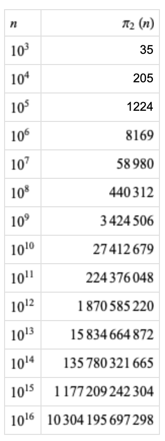
表示第  . 除了孪生素数本身之外,也有学者猜测,对于所有的正整数
  形如
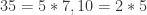
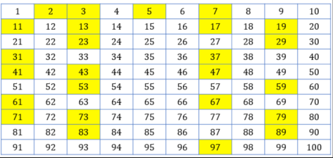
形如  的素数对同样有无穷多对。于是,在网上就有人对于有限的素数对进行了计算,让大家更好地看到素数之间的分布情况。
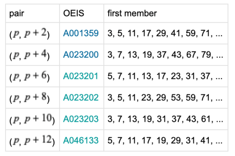
 使得
使得 

 ,随后这个结果被改进到 246。
 对于某个
对于某个  和无穷个
和无穷个  表示不大于
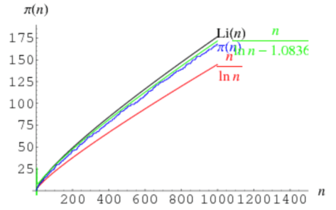
表示不大于  的所有素数的个数,那么
 表示不大于
表示不大于  使得
使得 

 ,那么
,那么  就是合数,但是它却不能被所有的素数
  整除,所以导致矛盾。因此素数是无穷多个。证明完毕。
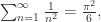
 并且
并且  也就是说,所有正整数的倒数和是发散的。
 通过欧拉公式可以得到:

 ,并且
,并且  ,
,  可以得到
可以得到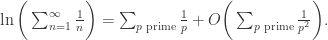

 这里,
这里,
 使得
使得  都是素数,那么
  ,进一步可以得到
 因此,孪生素数的倒数和是收敛的。证明完毕。
 的上界。同样的,也可以研究素数之间的间距究竟有多大,并且可以分析其量级大约是多少,此时就需要研究
![[1,x]](https://s0.wp.com/latex.php?latex=%5B1%2Cx%5D&bg=ffffff&fg=2b2b2b&s=0&c=20201002) 内,素数之间的最小间隔
内,素数之间的最小间隔  同时,素数之间的最大间隔
 个。于是把该区间
  的子区间,区间的个数为
  通过鸽笼原理 (Pigeonhole Principle) 可以得到此定理的结论。
 这
这 ![[n!+2, n!+n]](https://s0.wp.com/latex.php?latex=%5Bn%21%2B2%2C+n%21%2Bn%5D&bg=ffffff&fg=2b2b2b&s=0&c=20201002) 这个区间两侧。因此相邻素数的间隔没有上限,i.e.
这个区间两侧。因此相邻素数的间隔没有上限,i.e. 
![[2,n]](https://s0.wp.com/latex.php?latex=%5B2%2Cn%5D&bg=ffffff&fg=2b2b2b&s=0&c=20201002) 中的所有素数,则首先把
中的所有素数,则首先把  来排列,然后按照如下步骤执行:
 。
。
 其中
其中  ,
, ,
, 。
。 ,其中
,其中
 里面有
里面有  个不同的同余类,
 里面也有
里面也有  满足
满足  。也就是说
。也就是说  。令
。令  满足
满足  ,则有
,则有  。于是,
。于是, 。
。 是四个整数的平方和。于是必定存在一个最小的正整数
  使得
使得  使得
使得  为四个整数的平方和,不妨设为
  。
。 。
。 成立。令
成立。令  对于
对于  成立,并且
成立,并且  。因此,
。因此, 。令
。令  。因此,
。因此, 。
。 ,通过以上不等式得知
  等价于
等价于  对于
对于  。因此,
。因此, 矛盾。所以,
 成立。i.e.
  成立。
成立。 ,这里的
,这里的  正如恒定式里面所定义的。由于
  ,并且
,并且  。因此,
。因此, 对于
对于  ,
, 对于
对于  可以得到
可以得到  成立。但是,
 这与
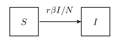
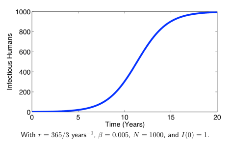
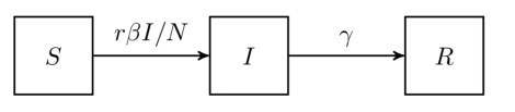
这与  上,可以定义以下几种人群:
 来表示;
来表示; 来表示;
来表示; 来表示;
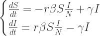
来表示; 。如果暂时不考虑人口增加和死亡的情况,那么
  是一个恒定的常数值。
 表示在单位时间内感染者接触到的易感者人数;
 表示感染者接触到易感者之后,易感者得病的概率;
 表示感染者康复的概率,有可能变成易感者(可再感染),也有可能变成康复者(不再感染)。
 是关于
是关于  和
和  ,那么它的解是:
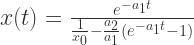 .
. 可以得到
可以得到 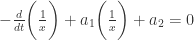 ;令
;令  ,得到
,得到  。所以,
。所以,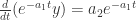 ,两边积分可以得到
  ,其中
,其中  。求解之后得到:
 。
。

 ,
, ,并且
,并且 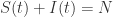 对于所有的
对于所有的  都成立。
都成立。 代入第二个微分方程可以得到:
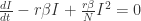 。因此根据前面所提到的常微分方程的解可以得到:
 .
. 这个定义。而
  ,所以,
,所以, ,从而
,从而  。
。
 ,其初始条件就是
  .
. 代入第二个微分方程可以得到:
 . 通过之前的 Claim 可以得到解为:
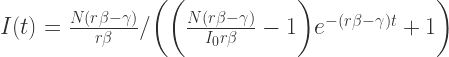 .
. 且
且  . 这个方程同样也是逻辑回归方程,只是它的渐近线与之前的 SI 模型有所不同。
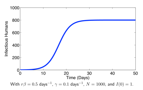
 。其初始条件是
  ,并且
,并且  和
和  对于所有的
对于所有的  ,于是
,于是  对于所有的
对于所有的 ![S_{\infty}\in[0,\infty]](https://s0.wp.com/latex.php?latex=S_%7B%5Cinfty%7D%5Cin%5B0%2C%5Cinfty%5D&bg=ffffff&fg=2b2b2b&s=0&c=20201002) 使得
使得  .
. ,因此对它两边积分得到
  . 左侧等于
  ,上界是
,上界是  ,因此令
,因此令  可以得到
可以得到  . 而
. 而  且是连续可微函数,因此
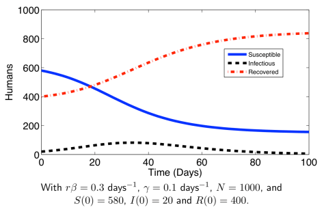
  。这意味着所有的感染人群都将康复。
 时,感染人数
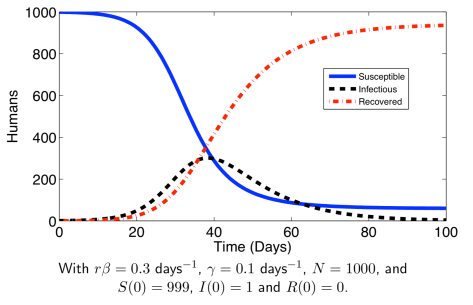

 。
。 是用以下符号来表示的:其中 sympy.exp() 表示以
  为底的函数。
 的小数值,可以使用 evalf() 函数,其中 evalf() 函数里面的值表示有效数字的位数。例如下面就是精确到 10 位有效数字。当然,也可以不输入。
 和
和  。
。 ,其中
,其中  和
和  都是多项式。一般情况下,我们希望对有理函数进行简化,合并或者分解的数学计算。
 并且去除公因子,那么可以使用 cancel 函数。另一个类似的就是 together 函数,但是不同之处在于 cancel 会消除公因子,together 不会消除公因子。例如:
 ,
, ,
, 。
。 出发,来介绍 SymPy 的各种函数使用方法。如果想进行变量替换,例如把
  ,那么可以使用 substitution 方法。除此之外,有的时候也希望能够得到函数
  在某个点的取值,例如
  ,那么可以把参数换成 1 即可得到函数的取值。例如,
 ,
,  ,
,  。
。 ,
, 。
。 这个概念了,但是在 SymPy 里面的写法还是一样的。
 ,
, ,
, 。
。 ,
, ,
, ,
, ,
, 。
。
 ,
, ,
, ,
, ,第二个矩阵表示
  ,
, 。
。 的解,可以有以下方案:
![I=[0,1]](https://s0.wp.com/latex.php?latex=I%3D%5B0%2C1%5D&bg=ffffff&fg=2b2b2b&s=0&c=20201002) 和开区间
和开区间  而言,在 SymPy 中使用以下方法来表示:
 在 SymPy 中用 sympy.S.Reals 来表示,自然数使用 sympy.S.Naturals,非负整数用 sympy.S.Naturals0,整数用 sympy.S.Integers 来表示。补集的计算可以用减号,也可以使用 complement 函数。
 来代表元素。&, |, ~, >> 分别表示 AND,OR,NOT,imply。而逻辑运算同样可以使用 sympy.simplify_logic 简化。
 ,
, 。
。 ,
, 。
。 ,
, ,
, ,
, 是一个二元函数,分别满足以下偏微分方程:
 ,
, ,
, 。
。
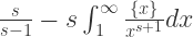
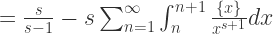
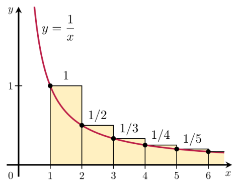
 根据级数与定积分的等价关系可以得到:
 时,
时,
 时,
时,
 上延拓到
上延拓到  上;
上; 上没有零点。
 上,就需要给出 Riemann Zeta 函数在
  上面,新的函数的取值必须与原函数的取值保持一致。
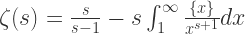 .
. 时,上述等式显然成立,两侧都是


 可以延拓到
可以延拓到  上。而且右侧的函数在
  是解析的,并且
  的解析函数,而且
  综上所述:
综上所述: 上是解析的;
 上。因此,数学家首先要找出的就是 Riemann Zeta 函数的非零区域。而本篇文章将会证明 Riemann Zeta 函数在
  上面没有零点。
 区域
区域


 ,当
,当  时,我们有
时,我们有


 when
when 

 直线
直线


 而对于其余的

 可以得到
可以得到


 换句话说
换句话说


 可以得到
可以得到

 对于所有的
对于所有的  成立。
成立。 存在阶数为
存在阶数为  其中
其中 
 并且
并且 


 可以得到左侧趋近于一个有限的值,但是右侧趋近于无穷,所以得到矛盾。也就是说当
  时,
时,  是
是  附近一个“狭长”的区域上,Riemann Zeta 函数没有零点。
 的方程。在复平面上,当复数
  时,
时,
 的形式和
的形式和  称为级数,里面的每一项都称为级数的通项。
 ,如果存在有限的 S 使得
  ,那么就称该级数收敛。否则,该级数就称为发散级数。
 收敛当且仅当对任意的
  ,存在
,存在  都有
都有  .
.


 也就是级数
也就是级数
 .
.
 的时候,公式是正确的。假设
  。计算可得:


 .
. 收敛。
收敛。


 当
当 
 ,都有
,都有  是发散的。
是发散的。 的取值。首先,我们回顾一下 Fourier 级数的一些性质:
 是一个关于
是一个关于  的周期函数, i.e.
  对于所有的
对于所有的  都成立。那么函数

 当
当 
 当
当 
 上满足 Lipschitz 条件,那么


 上的函数
上的函数  ,并且该函数是关于
  和
和  的公式,我们可以得到函数
 , 可以得到
 , 可以得到
 .
. .
.
 .
. , 得到
, 得到
 .
. = \sum\limits_{n=0}^{\infty} \lambda^n \cos(2\pi b^n x)")
 .
. = \sum\limits_{n=0}^{\infty} \lambda^n \phi(b^n x)")
 is a
is a  -periodic
  -function.
 because they are concrete examples of continuous but nowhere differentiable functions.
 tends to be a “fractal object” because
  = \phi(x) + \lambda f^{\phi}_{\lambda,b}(bx)")
 -function for all
  . In fact, for all
 ![{x,y\in[0,1]}](https://s0.wp.com/latex.php?latex=%7Bx%2Cy%5Cin%5B0%2C1%5D%7D&bg=ffffff&fg=000000&s=0 "{x,y\in[0,1]}") , we have
, we have - f^{\phi}_{\lambda,b}(y)}{|x-y|^{\alpha}} = \sum\limits_{n=0}^{\infty} \lambda^n b^{n\alpha} \left(\frac{\phi(b^n x) - \phi(b^n y)}{|b^n x - b^n y|^{\alpha}}\right),")
 - f^{\phi}_{\lambda,b}(y)}{|x-y|^{\alpha}} \leq \|\phi\|_{C^{\alpha}} \sum\limits_{n=0}^{\infty}(\lambda b^{\alpha})^n:=C(\phi,\alpha,\lambda,b) < \infty")
 , i.e.,
  .
.![{f:[0,1]\rightarrow\mathbb{R}}](https://s0.wp.com/latex.php?latex=%7Bf%3A%5B0%2C1%5D%5Crightarrow%5Cmathbb%7BR%7D%7D&bg=ffffff&fg=000000&s=0 "{f:[0,1]\rightarrow\mathbb{R}}") is
is)\leq 2 - \alpha")
 , the Hölder continuity condition
-f(y)|\leq C|x-y|^{\alpha}")
}") by the family
by the family _{j=1}^n}") of rectangles given by
of rectangles given by![\displaystyle R_{j,n}:=\left[\frac{j-1}{n}, \frac{j}{n}\right] \times \left[f(j/n)-\frac{C}{n^{\alpha}}, f(j/n)+\frac{C}{n^{\alpha}}\right]](https://s0.wp.com/latex.php?latex=%5Cdisplaystyle+R_%7Bj%2Cn%7D%3A%3D%5Cleft%5B%5Cfrac%7Bj-1%7D%7Bn%7D%2C+%5Cfrac%7Bj%7D%7Bn%7D%5Cright%5D+%5Ctimes+%5Cleft%5Bf%28j%2Fn%29-%5Cfrac%7BC%7D%7Bn%5E%7B%5Calpha%7D%7D%2C+f%28j%2Fn%29%2B%5Cfrac%7BC%7D%7Bn%5E%7B%5Calpha%7D%7D%5Cright%5D&bg=ffffff&fg=000000&s=0 "\displaystyle R_{j,n}:=\left[\frac{j-1}{n}, \frac{j}{n}\right] \times \left[f(j/n)-\frac{C}{n^{\alpha}}, f(j/n)+\frac{C}{n^{\alpha}}\right]")
}") . In fact, since
. In fact, since \leq 4C/n^{\alpha}}") for each
for each  , we have
^d\leq n\left(\frac{4C}{n^{\alpha}}\right)^d = (4C)^{1/\alpha} < \infty")
 . Because
 \leq 1/\alpha}") . Of course, this bound is certainly suboptimal for
. Of course, this bound is certainly suboptimal for  (because we know that
 \leq 2 < 1/\alpha}") anyway).Fortunately, we can refine the covering
anyway).Fortunately, we can refine the covering }") by taking into account that each rectangle
by taking into account that each rectangle  tends to be more vertical than horizontal (i.e., its height
  is usually larger than its width
  ). More precisely, we can divide each rectangle
  squares, say
 has diameter
  . In this way, we obtain a covering
 }") of
of  such that
^d \leq n\cdot n^{1-\alpha}\cdot\left(\frac{2}{n}\right)^d\leq (2C)^{2-\alpha}<\infty")
 . Since
 \leq 2-\alpha")
) = 2 + \frac{\log\lambda}{\log b} < 2")
) \geq 2 + \frac{\log\lambda}{\log b}")
 integer and for all
 ) = 2 + \frac{\log\lambda}{\log b}")
 a
a >1}") such that
such that) = 2 + \frac{\log\lambda}{\log b}")
 .
. such that
 .
. and
and  is large.
 = f^{\phi}_{\lambda,b}(x)}") for all
for all  . In particular, if
 }") is an invariant repeller for the endomorphism
is an invariant repeller for the endomorphism  given by
 = \left(bx\textrm{ mod }1, \frac{y-\phi(x)}{\lambda}\right)")
}") led Ledrappier to the following criterion for the validity of Mandelbrot’s conjecture when
led Ledrappier to the following criterion for the validity of Mandelbrot’s conjecture when  the alphabet
  . The unstable manifolds of
  through
 )")
 ,
,  , and
, and:=\sum\limits_{n=0}^{\infty} \gamma^n \phi'\left(\frac{x + u_1 + u_2 b + \dots + u_n b^{n-1}}{b^n}\right)")
)_*\mathbb{P}}") of the Bernoulli measure
of the Bernoulli measure  on
on  (induced by the discrete measure assigning weight
  to each letter of the alphabet
  of the expanding endomorphism
  ,
, = (bx\textrm{ mod }1, \gamma y + \psi(x)),")
 and
and =\phi'(x)}") . In plain terms, this means that
. In plain terms, this means that \ \ \ \ \ (1)")
 -invariant probability measure which is absolutely continuous along unstable manifolds (see
  have important consequences for the fractal geometry of the graph
 =1}") , i.e.,
, i.e.,)}{\log r} = 1 \textrm{ for } m_x\textrm{-a.e. } z")
}") has Hausdorff dimension
has Hausdorff dimension = 2 + \frac{\log\lambda}{\log b}")
\geq 2 + \frac{\log\lambda}{\log b}}") . By
. By  supported on
  := \textrm{ ess }\inf \underline{d}(\nu,x) \geq 2 + \frac{\log\lambda}{\log b}")
:=\liminf\limits_{r\rightarrow 0}\log \nu(B(x,r))/\log r}") . Finally, the main point is that the assumptions in Ledrappier theorem allow to prove that the measure
. Finally, the main point is that the assumptions in Ledrappier theorem allow to prove that the measure  given by the lift to
 ![{[0,1]}](https://s0.wp.com/latex.php?latex=%7B%5B0%2C1%5D%7D&bg=ffffff&fg=000000&s=0 "{[0,1]}") via the map
via the map )}") satisfies
satisfies \geq 2 + \frac{\log\lambda}{\log b}")
 , then
 for Lebesgue almost every
  for almost every
  implies that
 ,
,  and
and  , we say that two infinite words
  are
are }") -transverse at
-transverse at  if either
-s(x_0,v)|>\varepsilon")
-s'(x_0,v)|>\delta")
 ,
,  are
are  ,
,  are
are  ; otherwise, we say that
  and
and  are
are:= \{(k,l)\in\mathcal{A}^q\times\mathcal{A}^q: (k,l) \textrm{ is } (\varepsilon,\delta)\textrm{-tangent at } x_0\}}")
:=\bigcap\limits_{\varepsilon>0}\bigcap\limits_{\delta>0} E(q,x_0;\varepsilon,\delta)}") ;
;:=\max\limits_{k\in\mathcal{A}^q}\#\{l\in\mathcal{A}^q: (k,l)\in E(q,x_0)\}}")
:=\max\limits_{x_0\in\mathbb{R}/\mathbb{Z}} e(q,x_0)}") .
. integer such that
 <(\gamma b)^q}") , then
, then
 are mutually transverse, so that they almost fill a small neighborhood
  of some point
 and
and  , one has
 =1}") . Indeed, once we know that
. Indeed, once we know that  , they can apply Tsujii’s theorem and Ledrappier’s theorem (or rather Corollary
  = \cos(2\pi x)}") . If
. If  and
and <\gamma b")
 = 2+\frac{\log\lambda}{\log b}")
 ) requires the introduction of a modified version of Tsujii’s transversality condition: roughly speaking, Shen defines a function
 \leq e(q)}") (inspired from
(inspired from <(\gamma b)^q}") for some integer
for some integer  ;
; .
.:=-2\pi\sum\limits_{n=0}^{\infty} \gamma^n \sin\left(2\pi\frac{x + u_1 + u_2 b + \dots + u_n b^{n-1}}{b^n}\right)")
=-4\pi^2\sum\limits_{n=0}^{\infty} \left(\frac{\gamma}{b}\right)^n \cos\left(2\pi\frac{x + u_1 + u_2 b + \dots + u_n b^{n-1}}{b^n}\right)")
 , the series defining
 }") converges faster than the series defining
converges faster than the series defining }") .
.\in E(1,x_0)}") , then
, then - \sin\left(2\pi\frac{x_0+l}{b}\right)\right| \leq\frac{2\gamma}{1-\gamma} \ \ \ \ \ (2)")
 - \cos\left(2\pi\frac{x_0+l}{b}\right)\right| \leq \frac{2\gamma}{b-\gamma} \ \ \ \ \ (3)")
}") as follows. Take
as follows. Take =e(1,x_0)}") , and let
, and let  be such that
 ,\dots,(k,l_{e(1)})\in E(1,x_0)}") distinct elements listed in such a way that
distinct elements listed in such a way that\leq \sin(2\pi x_{i+1})")
-1}") , where
, where /b}") .
. - \cos\left(2\pi x_{i+1}\right)\right| \leq \frac{4\gamma}{b-\gamma}")
-\cos(2\pi x_{i+1}))^2 + (\sin(2\pi x_i)-\sin(2\pi x_{i+1}))^2 = 4\sin^2(\pi(x_i-x_{i+1}))\geq 4\sin^2(\pi/b),")
-\sin(2\pi x_{i+1})|\geq \sqrt{4\sin^2\left(\frac{\pi}{b}\right) - \left(\frac{4\gamma}{b-\gamma}\right)^2} \ \ \ \ \ (4)")
 - \left(\frac{4\gamma}{b-\gamma}\right)^2} > \frac{4}{b} \ \ \ \ \ (5)")
}") if
if }") ;
; ;
;}{\frac{4\gamma}{b-\gamma}}\rightarrow \frac{2\pi}{4\gamma} (< \frac{5}{3})}") as
as  , and
, and  - \frac{4\gamma}{b-\gamma} \rightarrow (2\pi-4\gamma)\frac{1}{b} (>\frac{2}{b})}") as
as  ).
).-\sin(2\pi x_{i+1})| > 4/b")
-1}") .
.\leq\sin(2\pi x_2)\leq\dots\leq\sin(2\pi x_{e(1)})\leq 1}") , the previous estimate implies that
, the previous estimate implies that-1)<\sum\limits_{i=1}^{e(1)-1}(\sin(2\pi x_{i+1}) - \sin(2\pi x_i)) = \sin(2\pi x_{e(1)}) - \sin(2\pi x_1)\leq 2,")
<1+\frac{b}{2}")
 ,
, <1+\frac{b}{2}<\gamma b")


 is symmetric if
  where
where ![\tau:[-1,1]\rightarrow [-1,1]](https://s0.wp.com/latex.php?latex=%5Ctau%3A%5B-1%2C1%5D%5Crightarrow+%5B-1%2C1%5D&bg=ffffff&fg=2b2b2b&s=0&c=20201002) is so that
is so that  and
and  if
if  . Furthermore, for each symmetric interval
 let
let  be the minimal positive integer with
  and let
 the Poincare map or transfer map to
 ![f:[-1,1]\rightarrow [-1,1]](https://s0.wp.com/latex.php?latex=f%3A%5B-1%2C1%5D%5Crightarrow+%5B-1%2C1%5D&bg=ffffff&fg=2b2b2b&s=0&c=20201002) be a unimodal map with one non-flat critical point with negative Schwarzian derivative and without attracting periodic points. Then there exists
be a unimodal map with one non-flat critical point with negative Schwarzian derivative and without attracting periodic points. Then there exists  and a sequence os symmetric intervals
  around the turning point which shrink to
  such that
  contains a
  scaled neighbourhood of
  and such that the following properties hold.
 is constant.
 be a component of the domain
  such that
  is monotone,
  and
and  . Here
  is the transfer time on
  .
. such that
 to
to  .
. can be written as
  where the distortion of
  is universally bounded by
  (Here
(Here  ) has either zero or full Lebesgue measure. An alternative way to define this notation of ergodicity goes as follows:
  such that
  has Lebesgue measure zero, at most one of these sets has positive Lebesgue measure. (Here
  .)
.) ,
,  for almost all
  (in which case it is called a solenoidal attractor);
 do not have such Cantor attractors. Moreover, Lyubich has shown that these absorbing Cantor attractors can not exist if the critical point is quadratic. However, Bruin, Keller, Nowicki and Van Strien showed that the absorbing Cantor attractors exist for Fibonacci maps when the critical order
  is sufficiently large enough.
 unimodal, has a quadratic critical point, has negative Schwarzian derivative and has no periodic attractors, then each closed forward invariant set
  to be the maximal interval on which
  is monotone. Let
  and
and  be the components of
  and define
  be the minimum of the length of
  and
and  .
. for almost all
  of
of  such that for almost every
  of
of  is monotone,
  and
and  .
. or
or 
 is
is  , with a bound on the first and the second derivatives. Assume that the interval
 ![[q_{0},q_{k}]](https://s0.wp.com/latex.php?latex=%5Bq_%7B0%7D%2Cq_%7Bk%7D%5D&bg=ffffff&fg=2b2b2b&s=0&c=20201002) ( or
( or ![[q_{0},q_{\infty}]](https://s0.wp.com/latex.php?latex=%5Bq_%7B0%7D%2Cq_%7B%5Cinfty%7D%5D&bg=ffffff&fg=2b2b2b&s=0&c=20201002) ) is positive invariant, so
) is positive invariant, so ![f(x)\in [q_{0},q_{k}]](https://s0.wp.com/latex.php?latex=f%28x%29%5Cin+%5Bq_%7B0%7D%2Cq_%7Bk%7D%5D&bg=ffffff&fg=2b2b2b&s=0&c=20201002) for all
for all ![x\in [q_{0}, q_{k}]](https://s0.wp.com/latex.php?latex=x%5Cin+%5Bq_%7B0%7D%2C+q_%7Bk%7D%5D&bg=ffffff&fg=2b2b2b&s=0&c=20201002) ( or
( or ![f(x)\in [q_{0},q_{\infty}]](https://s0.wp.com/latex.php?latex=f%28x%29%5Cin+%5Bq_%7B0%7D%2Cq_%7B%5Cinfty%7D%5D&bg=ffffff&fg=2b2b2b&s=0&c=20201002) for all
for all ![x\in[q_{0},q_{\infty}]](https://s0.wp.com/latex.php?latex=x%5Cin%5Bq_%7B0%7D%2Cq_%7B%5Cinfty%7D%5D&bg=ffffff&fg=2b2b2b&s=0&c=20201002) ).
). ( or
( or  ),assume that we have defined densities up to
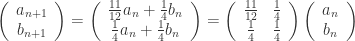
  , then define define
  as follows
 ,
,
 .
.
 on
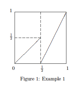
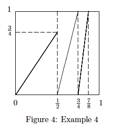
on ![[0,1]](https://s0.wp.com/latex.php?latex=%5B0%2C1%5D&bg=ffffff&fg=2b2b2b&s=0&c=20201002) . From the definition of
. From the definition of  , the slope on
  and
and  are 1 and 2, respectively. If
  , then it has only one pre-image on
  , then it has two pre-images, one is
  in
in  in
in 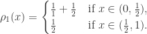


 , then


 . By induction,
  on
on  . Therefore,
  on
on 

 . By similar considerations,
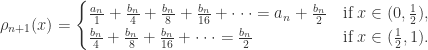

 and
and  for all


 and
and  for all
![A=[a_{ij}]](https://s0.wp.com/latex.php?latex=A%3D%5Ba_%7Bij%7D%5D&bg=ffffff&fg=2b2b2b&s=0&c=20201002) be a
be a  matrix. We say
  for all
  . Such a matrix is called irreducible if for any pair
  such that
  where
where  is the
  th element of
  . The matrix
  such that no eigenvalue of
  .
. and a non-negative right (column) eigenvector
  .
. ,
,  all
all  ).
). .
. has the largest absolute value in the set of all eigenvalues of
  for all pairs
  . That means
  is a strictly positive
  map
map  is called Markov if there exists a finite or countable family
  of disjoint open intervals in
  has Lebesgue measure zero and there exist
  such that for each
  and each interval
  such that
  is contained in one of the intervals
  one has
 , then
  ;
; such that
  for each
  . Usually, we will denote the Lebesgue measure of a Borel set
  .
. be corresponding partition. Then there exists a
  invariant probability measure
  on the Borel sets of
  is uniformly bounded and Holder continuous. Moreover, for each
  one has
  for some
  then
then for every Borel set
  .
. for each interval
  be a sequence of analytic functions on a domain
  which converges uniformly on compact subsets of
  converges uniformly on compact subsets to
  .
. . If
. If  for some
  , then for each
  , such that for all
  ,
,  has the same number of zeros in
  as does
  has no maximum in
  and analytic on the interior of
  is locally bounded on a domain
  , there is a positive number
  and a neighbourhood
  such that
  for all
  and all
  .
. form a locally bounded family in
  . However, the following partial converse does hold.
 is locally bounded and suppose that there is some
  for all
  and
and  .)
.) if, for each
  such that
  ,
,  whenever
  , for every
  if it is continuous (spherically continuous) at each point of
  is normal in
  contains either a subsequence which converges to a limit function
  uniformly on each compact subset of
  of continuous functions converges uniformly on a compact set
  such that for any
  ,
,  .
. exists for each
  which converges normally to an analytic function
  for each
  . Suppose, however, that
  , as well as a subsequence
  and points
  satisfying
 . Now
. Now  itself has a subsequence which converges uniformly on compact subsets to an analytic function
  , and
, and  from above. However, since
  on
on  . Then
  and such that no function of
  at more that
  in
in  . In the domain
  ,
,  is a normal family in
  but not compact.
 analytic in
  . Then
  . Then
  is a uniformly bounded family.
 analytic, univalent in
  . These are the normalised “Schlicht” functions in
  is normal and compact.
 . The point
  between
  and
and  is
is if
if  if
if  . Clearly,
  , and
, and  . The chordal metric and spherical metric are uniformly equivalent and generate the same open sets on the Riemann sphere.
 if, for any
  such that
  implies
  , for all
  contains a subsequence which converges spherically uniformly on compact subsets of
  in which
  or
or  uniformly as
  .
. . Then
  converges spherically on a point set
  is not a pole, the derivative in the spherical metric, called the spherical derivative, is given by
 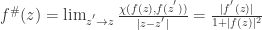 . If
. If  is a pole of
  .
. such that spherical derivative
  that is,
  is locally bounded.