
Introduction
Kaggle 是目前最大的 Data Scientist 聚集地。很多公司会拿出自家的数据并提供奖金,在 Kaggle 上组织数据竞赛。我最近完成了第一次比赛,在 2125 个参赛队伍中排名第 98 位(~ 5%)。因为是第一次参赛,所以对这个成绩我已经很满意了。在 Kaggle 上一次比赛的结果除了排名以外,还会显示的就是 Prize Winner,10% 或是 25% 这三档。所以刚刚接触 Kaggle 的人很多都会以 25% 或是 10% 为目标。在本文中,我试图根据自己第一次比赛的经验和从其他 Kaggler 那里学到的知识,为刚刚听说 Kaggle 想要参赛的新手提供一些切实可行的冲刺 10% 的指导。
本文的英文版见这里。

Kaggler 绝大多数都是用 Python 和 R 这两门语言的。因为我主要使用 Python,所以本文提到的例子都会根据 Python 来。不过 R 的用户应该也能不费力地了解到工具背后的思想。
首先简单介绍一些关于 Kaggle 比赛的知识:
- 不同比赛有不同的任务,分类、回归、推荐、排序等。比赛开始后训练集和测试集就会开放下载。
- 比赛通常持续 2 ~ 3 个月,每个队伍每天可以提交的次数有限,通常为 5 次。
- 比赛结束前一周是一个 Deadline,在这之后不能再组队,也不能再新加入比赛。所以想要参加比赛请务必在这一 Deadline 之前有过至少一次有效的提交。
- 一般情况下在提交后会立刻得到得分的反馈。不同比赛会采取不同的评分基准,可以在分数栏最上方看到使用的评分方法。
- 反馈的分数是基于测试集的一部分计算的,剩下的另一部分会被用于计算最终的结果。所以最后排名会变动。
- LB 指的就是在 Leaderboard 得到的分数,由上,有 Public LB 和 Private LB 之分。
- 自己做的 Cross Validation 得到的分数一般称为 CV 或是 Local CV。一般来说 CV 的结果比 LB 要可靠。
- 新手可以从比赛的 Forum 和 Scripts 中找到许多有用的经验和洞见。不要吝啬提问,Kaggler 都很热情。
那么就开始吧!
P.S. 本文假设读者对 Machine Learning 的基本概念和常见模型已经有一定了解。 Enjoy Reading!
General Approach
在这一节中我会讲述一次 Kaggle 比赛的大致流程。
Data Exploration
在这一步要做的基本就是 EDA (Exploratory Data Analysis),也就是对数据进行探索性的分析,从而为之后的处理和建模提供必要的结论。
通常我们会用 pandas 来载入数据,并做一些简单的可视化来理解数据。
Visualization
通常来说 matplotlib 和 seaborn 提供的绘图功能就可以满足需求了。
比较常用的图表有:
- 查看目标变量的分布。当分布不平衡时,根据评分标准和具体模型的使用不同,可能会严重影响性能。
- 对 Numerical Variable,可以用 Box Plot 来直观地查看它的分布。
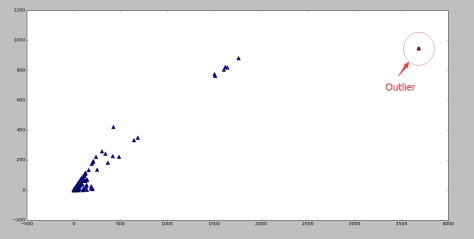
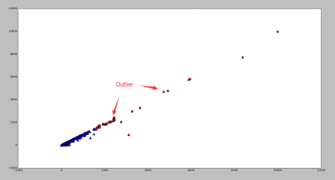
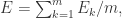
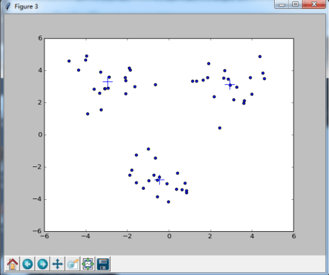
- 对于坐标类数据,可以用 Scatter Plot 来查看它们的分布趋势和是否有离群点的存在。
- 对于分类问题,将数据根据 Label 的不同着不同的颜色绘制出来,这对 Feature 的构造很有帮助。
- 绘制变量之间两两的分布和相关度图表。
这里有一个在著名的 Iris 数据集上做了一系列可视化的例子,非常有启发性。
Statistical Tests
我们可以对数据进行一些统计上的测试来验证一些假设的显著性。虽然大部分情况下靠可视化就能得到比较明确的结论,但有一些定量结果总是更理想的。不过,在实际数据中经常会遇到非 i.i.d. 的分布。所以要注意测试类型的的选择和对显著性的解释。
在某些比赛中,由于数据分布比较奇葩或是噪声过强,Public LB 的分数可能会跟Local CV 的结果相去甚远。可以根据一些统计测试的结果来粗略地建立一个阈值,用来衡量一次分数的提高究竟是实质的提高还是由于数据的随机性导致的。
Data Preprocessing
大部分情况下,在构造 Feature 之前,我们需要对比赛提供的数据集进行一些处理。通常的步骤有:
- 有时数据会分散在几个不同的文件中,需要 Join 起来。
- 处理 Missing Data。
- 处理 Outlier。
- 必要时转换某些 Categorical Variable 的表示方式。
- 有些 Float 变量可能是从未知的 Int 变量转换得到的,这个过程中发生精度损失会在数据中产生不必要的 Noise,即两个数值原本是相同的却在小数点后某一位开始有不同。这对 Model 可能会产生很负面的影响,需要设法去除或者减弱 Noise。
这一部分的处理策略多半依赖于在前一步中探索数据集所得到的结论以及创建的可视化图表。在实践中,我建议使用 iPython Notebook 进行对数据的操作,并熟练掌握常用的 pandas 函数。这样做的好处是可以随时得到结果的反馈和进行修改,也方便跟其他人进行交流(在 Data Science 中 Reproducible Results 是很重要的)。
下面给两个例子。
Outlier

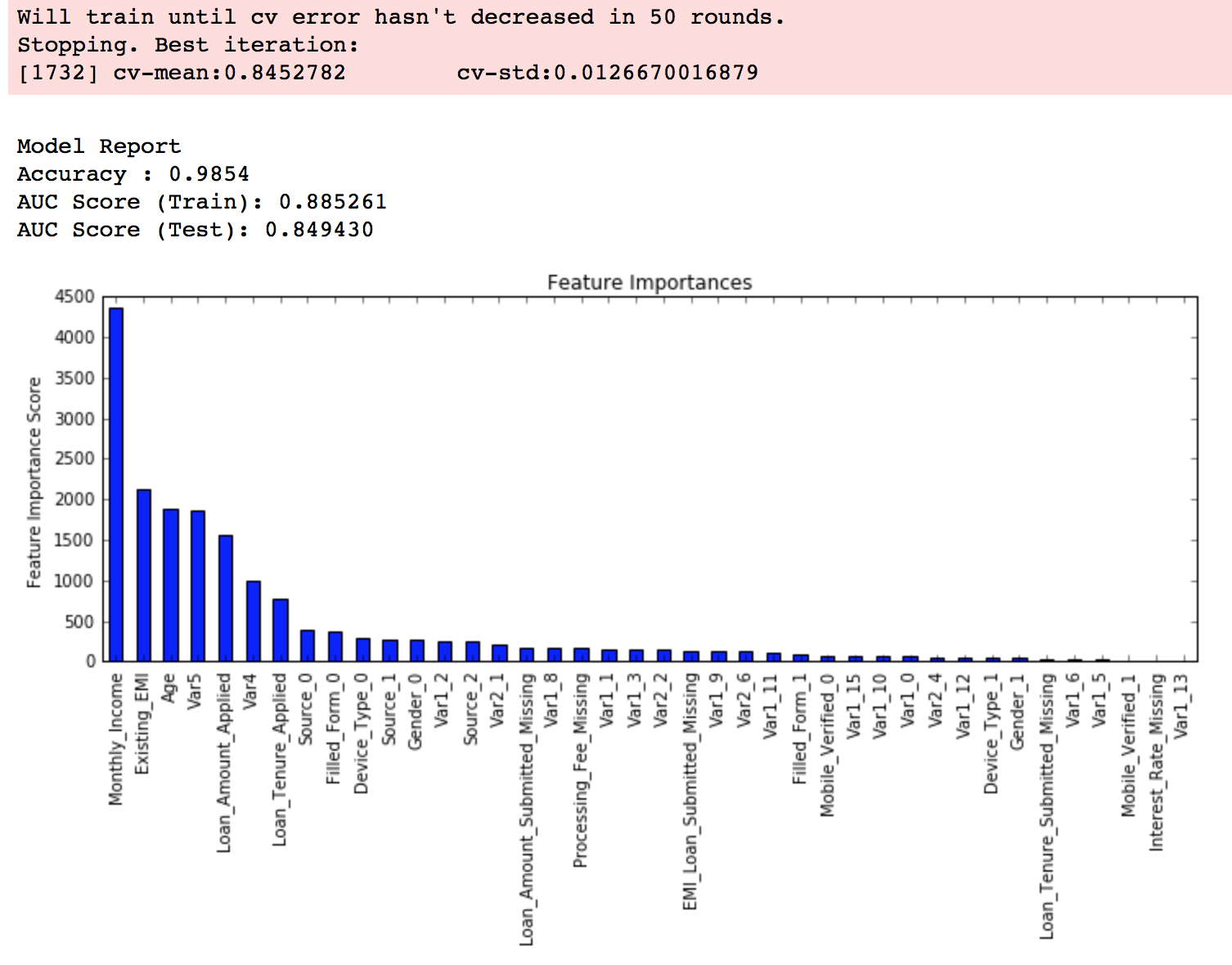
这是经过 Scaling 的坐标数据。可以发现右上角存在一些离群点,去除以后分布比较正常。
Dummy Variables
对于 Categorical Variable,常用的做法就是 One-hot encoding。即对这一变量创建一组新的伪变量,对应其所有可能的取值。这些变量中只有这条数据对应的取值为 1,其他都为 0。
如下,将原本有 7 种可能取值的 Weekdays 变量转换成 7 个 Dummy Variables。

要注意,当变量可能取值的范围很大(比如一共有成百上千类)时,这种简单的方法就不太适用了。这时没有有一个普适的方法,但我会在下一小节描述其中一种。
Feature Engineering
有人总结 Kaggle 比赛是 “Feature 为主,调参和 Ensemble 为辅”,我觉得很有道理。Feature Engineering 能做到什么程度,取决于对数据领域的了解程度。比如在数据包含大量文本的比赛中,常用的 NLP 特征就是必须的。怎么构造有用的 Feature,是一个不断学习和提高的过程。
一般来说,当一个变量从直觉上来说对所要完成的目标有帮助,就可以将其作为 Feature。至于它是否有效,最简单的方式就是通过图表来直观感受。比如:

Feature Selection
总的来说,我们应该生成尽量多的 Feature,相信 Model 能够挑出最有用的 Feature。但有时先做一遍 Feature Selection 也能带来一些好处:
- Feature 越少,训练越快。
- 有些 Feature 之间可能存在线性关系,影响 Model 的性能。
- 通过挑选出最重要的 Feature,可以将它们之间进行各种运算和操作的结果作为新的 Feature,可能带来意外的提高。
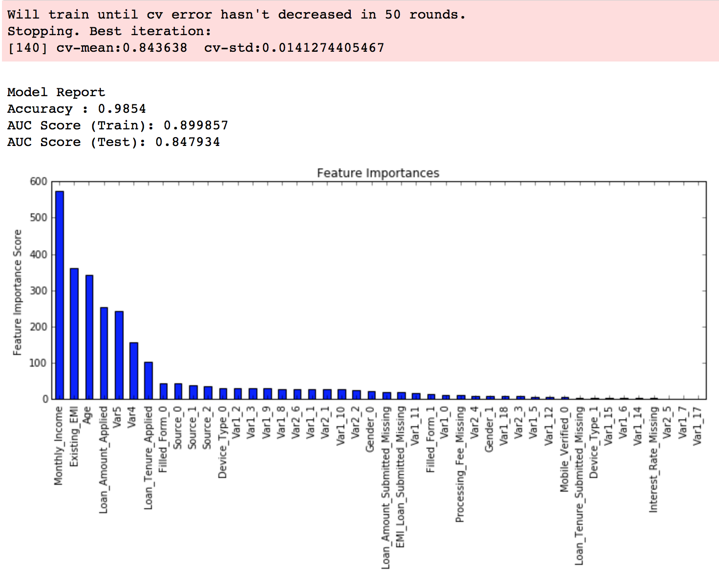
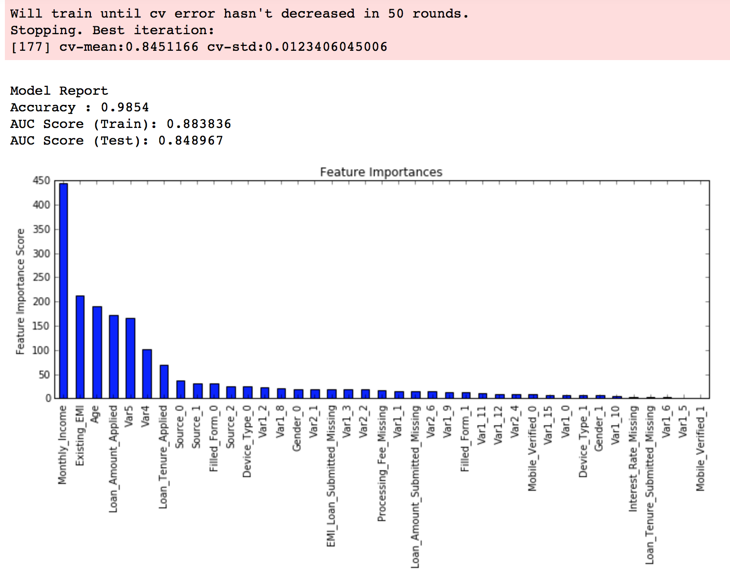
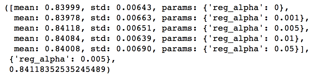
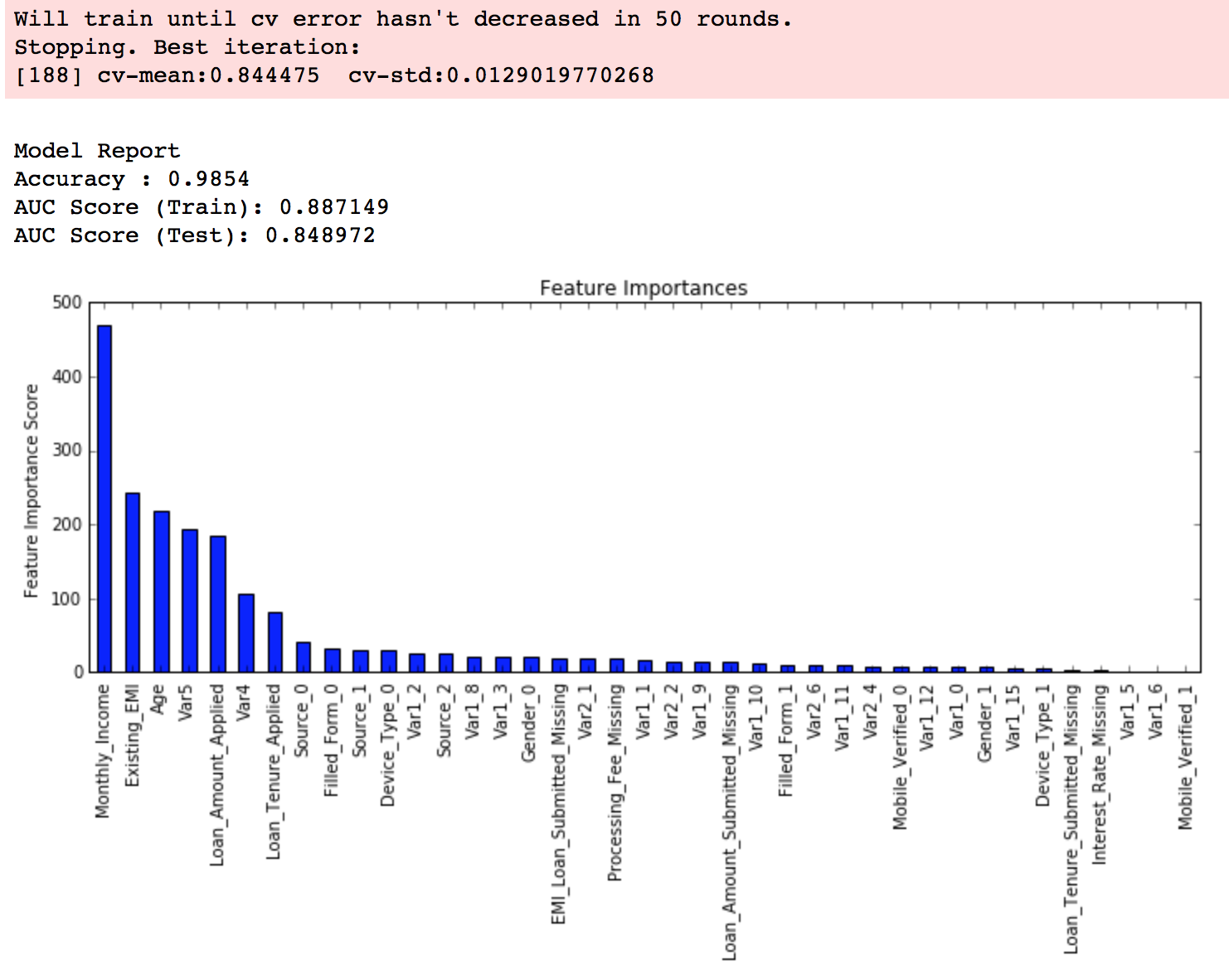
Feature Selection 最实用的方法也就是看 Random Forest 训练完以后得到的Feature Importance 了。其他有一些更复杂的算法在理论上更加 Robust,但是缺乏实用高效的实现,比如这个。从原理上来讲,增加 Random Forest 中树的数量可以在一定程度上加强其对于 Noisy Data 的 Robustness。
看 Feature Importance 对于某些数据经过脱敏处理的比赛尤其重要。这可以免得你浪费大把时间在琢磨一个不重要的变量的意义上。
Feature Encoding
这里用一个例子来说明在一些情况下 Raw Feature 可能需要经过一些转换才能起到比较好的效果。
假设有一个 Categorical Variable 一共有几万个取值可能,那么创建 Dummy Variables 的方法就不可行了。这时一个比较好的方法是根据 Feature Importance 或是这些取值本身在数据中的出现频率,为最重要(比如说前 95% 的 Importance)那些取值(有很大可能只有几个或是十几个)创建 Dummy Variables,而所有其他取值都归到一个“其他”类里面。
Model Selection
准备好 Feature 以后,就可以开始选用一些常见的模型进行训练了。Kaggle 上最常用的模型基本都是基于树的模型:
- Gradient Boosting
- Random Forest
- Extra Randomized Trees
以下模型往往在性能上稍逊一筹,但是很适合作为 Ensemble 的 Base Model。这一点之后再详细解释。(当然,在跟图像有关的比赛中神经网络的重要性还是不能小觑的。)
- SVM
- Linear Regression
- Logistic Regression
- Neural Networks
以上这些模型基本都可以通过 sklearn 来使用。
当然,这里不能不提一下 Xgboost。Gradient Boosting 本身优秀的性能加上Xgboost 高效的实现,使得它在 Kaggle 上广为使用。几乎每场比赛的获奖者都会用 Xgboost 作为最终 Model 的重要组成部分。在实战中,我们往往会以 Xgboost 为主来建立我们的模型并且验证 Feature 的有效性。顺带一提,在 Windows 上安装 Xgboost 很容易遇到问题,目前已知最简单、成功率最高的方案可以参考我在这篇帖子中的描述。
Model Training
在训练时,我们主要希望通过调整参数来得到一个性能不错的模型。一个模型往往有很多参数,但其中比较重要的一般不会太多。比如对 sklearn 的 RandomForestClassifier 来说,比较重要的就是随机森林中树的数量 n_estimators 以及在训练每棵树时最多选择的特征数量 max_features。所以我们需要对自己使用的模型有足够的了解,知道每个参数对性能的影响是怎样的。
通常我们会通过一个叫做 Grid Search 的过程来确定一组最佳的参数。其实这个过程说白了就是根据给定的参数候选对所有的组合进行暴力搜索。
|
1
2
3
|
param_grid = {‘n_estimators’: [300, 500], ‘max_features’: [10, 12, 14]}
model = grid_search.GridSearchCV(estimator=rfr, param_grid=param_grid, n_jobs=1, cv=10, verbose=20, scoring=RMSE)
model.fit(X_train, y_train)
|
顺带一提,Random Forest 一般在 max_features 设为 Feature 数量的平方根附近得到最佳结果。
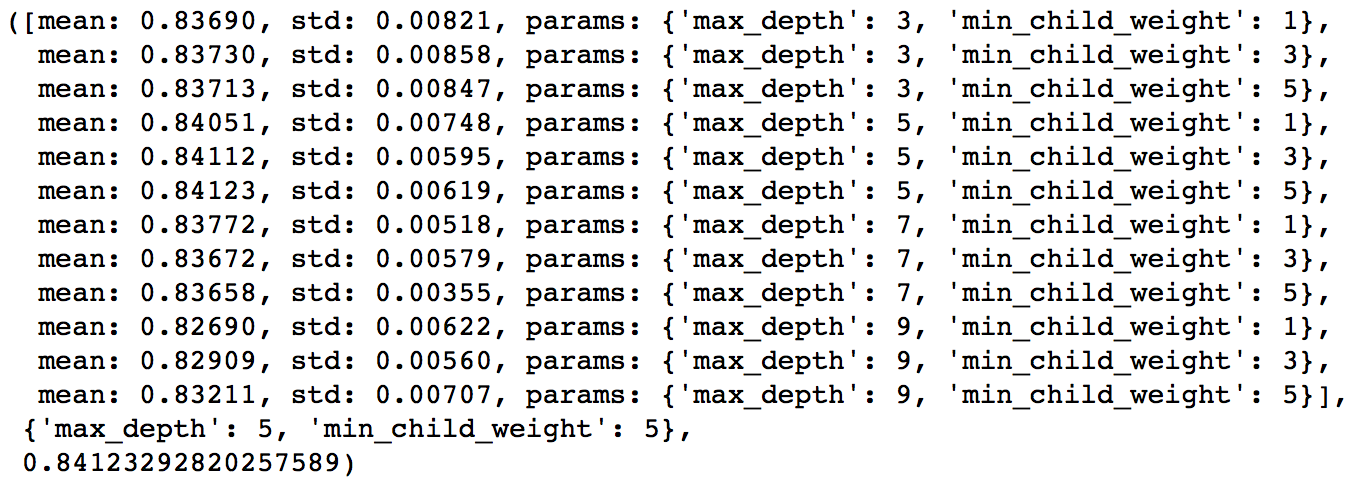
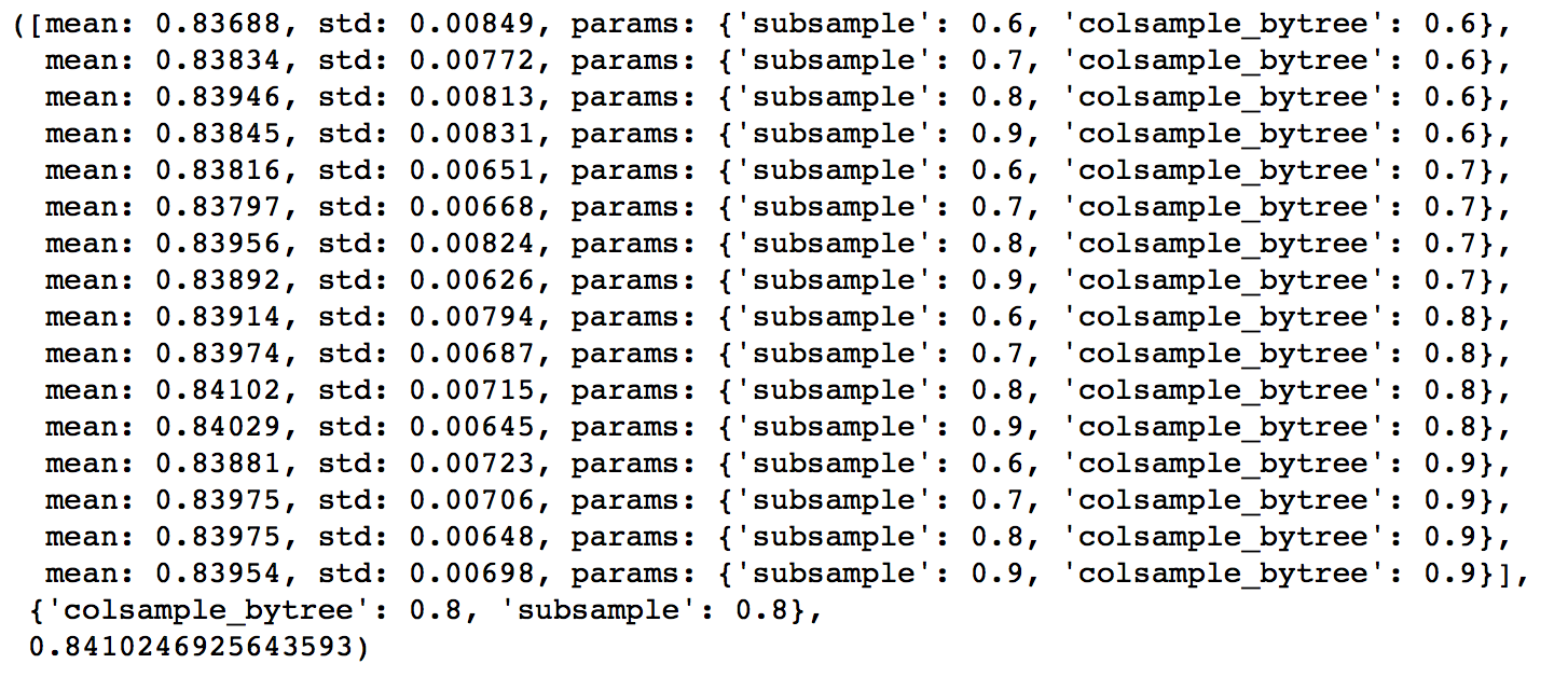
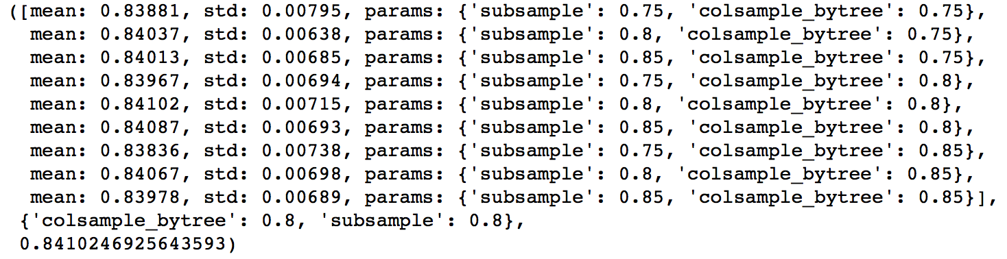
这里要重点讲一下 Xgboost 的调参。通常认为对它性能影响较大的参数有:
eta:每次迭代完成后更新权重时的步长。越小训练越慢。num_round:总共迭代的次数。subsample:训练每棵树时用来训练的数据占全部的比例。用于防止 Overfitting。colsample_bytree:训练每棵树时用来训练的特征的比例,类似RandomForestClassifier的max_features。max_depth:每棵树的最大深度限制。与 Random Forest 不同,Gradient Boosting 如果不对深度加以限制,最终是会 Overfit 的。early_stopping_rounds:用于控制在 Out Of Sample 的验证集上连续多少个迭代的分数都没有提高后就提前终止训练。用于防止 Overfitting。
一般的调参步骤是:
- 将训练数据的一部分划出来作为验证集。
- 先将
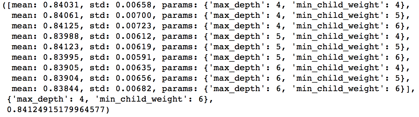
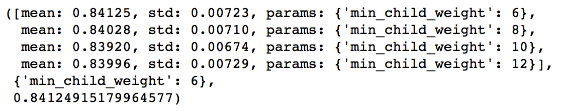
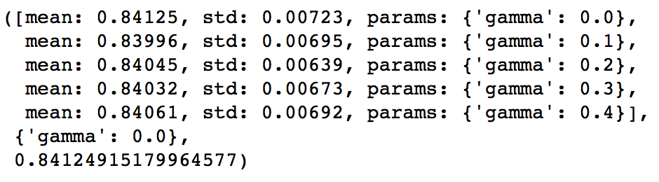
eta设得比较高(比如 0.1),num_round设为 300 ~ 500。 - 用 Grid Search 对其他参数进行搜索
- 逐步将
eta降低,找到最佳值。 - 以验证集为 watchlist,用找到的最佳参数组合重新在训练集上训练。注意观察算法的输出,看每次迭代后在验证集上分数的变化情况,从而得到最佳的
early_stopping_rounds。
|
1
2
3
4
5
6
7
8
9
10
11
12
13
14
15
16
17
|
X_dtrain, X_deval, y_dtrain, y_deval = cross_validation.train_test_split(X_train, y_train, random_state=1026, test_size=0.3)
dtrain = xgb.DMatrix(X_dtrain, y_dtrain)
deval = xgb.DMatrix(X_deval, y_deval)
watchlist = [(deval, ‘eval’)]
params = {
‘booster’: ‘gbtree’,
‘objective’: ‘reg:linear’,
‘subsample’: 0.8,
‘colsample_bytree’: 0.85,
‘eta’: 0.05,
‘max_depth’: 7,
‘seed’: 2016,
‘silent’: 0,
‘eval_metric’: ‘rmse’
}
clf = xgb.train(params, dtrain, 500, watchlist, early_stopping_rounds=50)
pred = clf.predict(xgb.DMatrix(df_test))
|
最后要提一点,所有具有随机性的 Model 一般都会有一个 seed 或是 random_state 参数用于控制随机种子。得到一个好的 Model 后,在记录参数时务必也记录下这个值,从而能够在之后重现 Model。
Cross Validation
Cross Validation 是非常重要的一个环节。它让你知道你的 Model 有没有 Overfit,是不是真的能够 Generalize 到测试集上。在很多比赛中 Public LB 都会因为这样那样的原因而不可靠。当你改进了 Feature 或是 Model 得到了一个更高的 CV 结果,提交之后得到的 LB 结果却变差了,一般认为这时应该相信 CV 的结果。当然,最理想的情况是多种不同的 CV 方法得到的结果和 LB 同时提高,但这样的比赛并不是太多。
在数据的分布比较随机均衡的情况下,5-Fold CV 一般就足够了。如果不放心,可以提到 10-Fold。但是 Fold 越多训练也就会越慢,需要根据实际情况进行取舍。
很多时候简单的 CV 得到的分数会不大靠谱,Kaggle 上也有很多关于如何做 CV 的讨论。比如这个。但总的来说,靠谱的 CV 方法是 Case By Case 的,需要在实际比赛中进行尝试和学习,这里就不再(也不能)叙述了。
Ensemble Generation
Ensemble Learning 是指将多个不同的 Base Model 组合成一个 Ensemble Model 的方法。它可以同时降低最终模型的 Bias 和 Variance(证明可以参考这篇论文,我最近在研究类似的理论,可能之后会写新文章详述),从而在提高分数的同时又降低 Overfitting 的风险。在现在的 Kaggle 比赛中要不用 Ensemble 就拿到奖金几乎是不可能的。
常见的 Ensemble 方法有这么几种:
- Bagging:使用训练数据的不同随机子集来训练每个 Base Model,最后进行每个 Base Model 权重相同的 Vote。也即 Random Forest 的原理。
- Boosting:迭代地训练 Base Model,每次根据上一个迭代中预测错误的情况修改训练样本的权重。也即 Gradient Boosting 的原理。比 Bagging 效果好,但更容易 Overfit。
- Blending:用不相交的数据训练不同的 Base Model,将它们的输出取(加权)平均。实现简单,但对训练数据利用少了。
- Stacking:接下来会详细介绍。
从理论上讲,Ensemble 要成功,有两个要素:
- Base Model 之间的相关性要尽可能的小。这就是为什么非 Tree-based Model 往往表现不是最好但还是要将它们包括在 Ensemble 里面的原因。Ensemble 的 Diversity 越大,最终 Model 的 Bias 就越低。
- Base Model 之间的性能表现不能差距太大。这其实是一个 Trade-off,在实际中很有可能表现相近的 Model 只有寥寥几个而且它们之间相关性还不低。但是实践告诉我们即使在这种情况下 Ensemble 还是能大幅提高成绩。
Stacking
相比 Blending,Stacking 能更好地利用训练数据。以 5-Fold Stacking 为例,它的基本原理如图所示:

整个过程很像 Cross Validation。首先将训练数据分为 5 份,接下来一共 5 个迭代,每次迭代时,将 4 份数据作为 Training Set 对每个 Base Model 进行训练,然后在剩下一份 Hold-out Set 上进行预测。同时也要将其在测试数据上的预测保存下来。这样,每个 Base Model 在每次迭代时会对训练数据的其中 1 份做出预测,对测试数据的全部做出预测。5 个迭代都完成以后我们就获得了一个 #训练数据行数 x #Base Model 数量 的矩阵,这个矩阵接下来就作为第二层的 Model 的训练数据。当第二层的 Model 训练完以后,将之前保存的 Base Model 对测试数据的预测(因为每个 Base Model 被训练了 5 次,对测试数据的全体做了 5 次预测,所以对这 5 次求一个平均值,从而得到一个形状与第二层训练数据相同的矩阵)拿出来让它进行预测,就得到最后的输出。
这里给出我的实现代码:
|
1
2
3
4
5
6
7
8
9
10
11
12
13
14
15
16
17
18
19
20
21
22
23
24
25
26
27
28
29
30
31
32
33
34
|
class Ensemble(object):
def __init__(self, n_folds, stacker, base_models):
self.n_folds = n_folds
self.stacker = stacker
self.base_models = base_models
def fit_predict(self, X, y, T):
X = np.array(X)
y = np.array(y)
T = np.array(T)
folds = list(KFold(len(y), n_folds=self.n_folds, shuffle=True, random_state=2016))
S_train = np.zeros((X.shape[0], len(self.base_models)))
S_test = np.zeros((T.shape[0], len(self.base_models)))
for i, clf in enumerate(self.base_models):
S_test_i = np.zeros((T.shape[0], len(folds)))
for j, (train_idx, test_idx) in enumerate(folds):
X_train = X[train_idx]
y_train = y[train_idx]
X_holdout = X[test_idx]
# y_holdout = y[test_idx]
clf.fit(X_train, y_train)
y_pred = clf.predict(X_holdout)[:]
S_train[test_idx, i] = y_pred
S_test_i[:, j] = clf.predict(T)[:]
S_test[:, i] = S_test_i.mean(1)
self.stacker.fit(S_train, y)
y_pred = self.stacker.predict(S_test)[:]
return y_pred
|
获奖选手往往会使用比这复杂得多的 Ensemble,会出现三层、四层甚至五层,不同的层数之间有各种交互,还有将经过不同的 Preprocessing 和不同的 Feature Engineering 的数据用 Ensemble 组合起来的做法。但对于新手来说,稳稳当当地实现一个正确的 5-Fold Stacking 已经足够了。
*Pipeline
可以看出 Kaggle 比赛的 Workflow 还是比较复杂的。尤其是 Model Selection 和 Ensemble。理想情况下,我们需要搭建一个高自动化的 Pipeline,它可以做到:
- 模块化 Feature Transform,只需写很少的代码就能将新的 Feature 更新到训练集中。
- 自动化 Grid Search,只要预先设定好使用的 Model 和参数的候选,就能自动搜索并记录最佳的 Model。
- 自动化 Ensemble Generation,每个一段时间将现有最好的 K 个 Model 拿来做 Ensemble。
对新手来说,第一点可能意义还不是太大,因为 Feature 的数量总是人脑管理的过来的;第三点问题也不大,因为往往就是在最后做几次 Ensemble。但是第二点还是很有意义的,手工记录每个 Model 的表现不仅浪费时间而且容易产生混乱。
Crowdflower Search Results Relevance 的第一名获得者 Chenglong Chen 将他在比赛中使用的 Pipeline 公开了,非常具有参考和借鉴意义。只不过看懂他的代码并将其中的逻辑抽离出来搭建这样一个框架,还是比较困难的一件事。可能在参加过几次比赛以后专门抽时间出来做会比较好。
Home Depot Search Relevance
在这一节中我会具体分享我在 Home Depot Search Relevance 比赛中是怎么做的,以及比赛结束后从排名靠前的队伍那边学到的做法。
首先简单介绍这个比赛。Task 是判断用户搜索的关键词和网站返回的结果之间的相关度有多高。相关度是由 3 个人类打分取平均得到的,每个人可能打 1 ~ 3 分,所以这是一个回归问题。数据中包含用户的搜索词,返回的产品的标题和介绍,以及产品相关的一些属性比如品牌、尺寸、颜色等。使用的评分基准是 RMSE。
这个比赛非常像 Crowdflower Search Results Relevance 那场比赛。不过那边用的评分基准是 Quadratic Weighted Kappa,把 1 误判成 4 的惩罚会比把 1 判成 2 的惩罚大得多,所以在最后 Decode Prediction 的时候会更麻烦一点。除此以外那次比赛没有提供产品的属性。
EDA
由于加入比赛比较晚,当时已经有相当不错的 EDA 了。尤其是这个。从中我得到的启发有:
- 同一个搜索词/产品都出现了多次,数据分布显然不 i.i.d.。
- 文本之间的相似度很有用。
- 产品中有相当大一部分缺失属性,要考虑这会不会使得从属性中得到的 Feature 反而难以利用。
- 产品的 ID 对预测相关度很有帮助,但是考虑到训练集和测试集之间的重叠度并不太高,利用它会不会导致 Overfitting?
Preprocessing
这次比赛中我的 Preprocessing 和 Feature Engineering 的具体做法都可以在这里看到。我只简单总结一下和指出重要的点。
- 利用 Forum 上的 Typo Dictionary 修正搜索词中的错误。
- 统计属性的出现次数,将其中出现次数多又容易利用的记录下来。
- 将训练集和测试集合并,并与产品描述和属性 Join 起来。这是考虑到后面有一系列操作,如果不合并的话就要重复写两次了。
- 对所有文本能做 Stemming 和 Tokenizing,同时手工做了一部分格式统一化(比如涉及到数字和单位的)和同义词替换。
Feature
- *Attribute Features
- 是否包含某个特定的属性(品牌、尺寸、颜色、重量、内用/外用、是否有能源之星认证等)
- 这个特定的属性是否匹配
- Meta Features
- 各个文本域的长度
- 是否包含属性域
- 品牌(将所有的品牌做数值离散化)
- 产品 ID
- 简单匹配
- 搜索词是否在产品标题、产品介绍或是产品属性中出现
- 搜索词在产品标题、产品介绍或是产品属性中出现的数量和比例
- *搜索词中的第 i 个词是否在产品标题、产品介绍或是产品属性中出现
- 搜索词和产品标题、产品介绍以及产品属性之间的文本相似度
- BOW Cosine Similairty
- TF-IDF Cosine Similarity
- Jaccard Similarity
- *Edit Distance
- Word2Vec Distance(由于效果不好,最后没有使用,但似乎是因为用的不对)
- Latent Semantic Indexing:通过将 BOW/TF-IDF Vectorization 得到的矩阵进行 SVD 分解,我们可以得到不同搜索词/产品组合的 Latent 标识。这个 Feature 使得 Model 能够在一定程度上对不同的组合做出区别,从而解决某些产品缺失某些 Feature 的问题。
值得一提的是,上面打了 * 的 Feature 都是我在最后一批加上去的。问题是,使用这批 Feature 训练得到的 Model 反而比之前的要差,而且还差不少。我一开始是以为因为 Feature 的数量变多了所以一些参数需要重新调优,但在浪费了很多时间做 Grid Search 以后却发现还是没法超过之前的分数。这可能就是之前提到的 Feature 之间的相互作用导致的问题。当时我设想过一个看到过好几次的解决方案,就是将使用不同版本 Feature 的 Model 通过 Ensemble 组合起来。但最终因为时间关系没有实现。事实上排名靠前的队伍分享的解法里面基本都提到了将不同的 Preprocessing 和 Feature Engineering 做 Ensemble 是获胜的关键。
Model
我一开始用的是 RandomForestRegressor,后来在 Windows 上折腾 Xgboost 成功了就开始用 XGBRegressor。XGB 的优势非常明显,同样的数据它只需要不到一半的时间就能跑完,节约了很多时间。
比赛中后期我基本上就是一边台式机上跑 Grid Search,一边在笔记本上继续研究 Feature。
这次比赛数据分布很不独立,所以期间多次遇到改进的 Feature 或是 Grid Search新得到的参数训练出来的模型反而 LB 分数下降了。由于被很多前辈教导过要相信自己的 CV,我的决定是将 5-Fold 提到 10-Fold,然后以 CV 为标准继续前进。
Ensemble
最终我的 Ensemble 的 Base Model 有以下四个:
RandomForestRegressorExtraTreesRegressorGradientBoostingRegressorXGBRegressor
第二层的 Model 还是用的 XGB。
因为 Base Model 之间的相关都都太高了(最低的一对也有 0.9),我原本还想引入使用 gblinear 的 XGBRegressor 以及 SVR,但前者的 RMSE 比其他几个 Model 高了 0.02(这在 LB 上有几百名的差距),而后者的训练实在太慢了。最后还是只用了这四个。
值得一提的是,在开始做 Stacking 以后,我的 CV 和 LB 成绩的提高就是完全同步的了。
在比赛最后两天,因为身心疲惫加上想不到还能有什么显著的改进,我做了一件事情:用 20 个不同的随机种子来生成 Ensemble,最后取 Weighted Average。这个其实算是一种变相的 Bagging。其意义在于按我实现 Stacking 的方式,我在训练 Base Model 时只用了 80% 的训练数据,而训练第二层的 Model 时用了 100% 的数据,这在一定程度上增大了 Overfitting 的风险。而每次更改随机种子可以确保每次用的是不同的 80%,这样在多次训练取平均以后就相当于逼近了使用 100% 数据的效果。这给我带来了大约 0.0004 的提高,也很难受说是真的有效还是随机性了。
比赛结束后我发现我最好的单个 Model 在 Private LB 上的得分是 0.46378,而最终 Stacking 的得分是 0.45849。这是 174 名和 98 名的差距。也就是说,我单靠 Feature 和调参进到了 前 10%,而 Stacking 使我进入了前 5%。
Lessons Learned
比赛结束后一些队伍分享了他们的解法,从中我学到了一些我没有做或是做的不够好的地方:
- 产品标题的组织方式是有 Pattern 的,比如一个产品是否带有某附件一定会用
With/Without XXX的格式放在标题最后。 - 使用外部数据,比如 WordNet,Reddit 评论数据集等来训练同义词和上位词(在一定程度上替代 Word2Vec)词典。
- 基于字母而不是单词的 NLP Feature。这一点我让我十分费解,但请教以后发现非常有道理。举例说,排名第三的队伍在计算匹配度时,将搜索词和内容中相匹配的单词的长度也考虑进去了。这是因为他们发现越长的单词约具体,所以越容易被用户认为相关度高。此外他们还使用了逐字符的序列比较(
difflib.SequenceMatcher),因为这个相似度能够衡量视觉上的相似度。像这样的 Feature 的确不是每个人都能想到的。 - 标注单词的词性,找出中心词,计算基于中心词的各种匹配度和距离。这一点我想到了,但没有时间尝试。
- 将产品标题/介绍中 TF-IDF 最高的一些 Trigram 拿出来,计算搜索词中出现在这些 Trigram 中的比例;反过来以搜索词为基底也做一遍。这相当于是从另一个角度抽取了一些 Latent 标识。
- 一些新颖的距离尺度,比如 Word Movers Distance
- 除了 SVD 以外还可以用上 NMF。
- 最重要的 Feature 之间的 Pairwise Polynomial Interaction。
- 针对数据不 i.i.d. 的问题,在 CV 时手动构造测试集与验证集之间产品 ID 不重叠和重叠的两种不同分割,并以与实际训练集/测试集的分割相同的比例来做 CV 以逼近 LB 的得分分布。
至于 Ensemble 的方法,我暂时还没有办法学到什么,因为自己只有最简单的 Stacking 经验。
Summary
Takeaways
- 比较早的时候就开始做 Ensemble 是对的,这次比赛到倒数第三天我还在纠结 Feature。
- 很有必要搭建一个 Pipeline,至少要能够自动训练并记录最佳参数。
- Feature 为王。我花在 Feature 上的时间还是太少。
- 可能的话,多花点时间去手动查看原始数据中的 Pattern。
Issues Raised
我认为在这次比赛中遇到的一些问题是很有研究价值的:
- 在数据分布并不 i.i.d. 甚至有 Dependency 时如何做靠谱的 CV。
- 如何量化 Ensemble 中 Diversity vs. Accuracy 的 Trade-off。
- 如何处理 Feature 之间互相影响导致性能反而下降。
Beginner Tips
给新手的一些建议:
- 选择一个感兴趣的比赛。如果你对相关领域原本就有一些洞见那就更理想了。
- 根据我描述的方法开始探索、理解数据并进行建模。
- 通过 Forum 和 Scripts 学习其他人对数据的理解和构建 Feature 的方式。
- 如果之前有过类似的比赛,可以去找当时获奖者的 Interview 和 Blog Post 作为参考,往往很有用。
- 在得到一个比较不错的 LB 分数(比如已经接近前 10%)以后可以开始尝试做 Ensemble。
- 如果觉得自己有希望拿到奖金,开始找人组队吧!
- 到比赛结束为止要绷紧一口气不能断,尽量每天做一些新尝试。
- 比赛结束后学习排名靠前的队伍的方法,思考自己这次比赛中的不足和发现的问题,可能的话再花点时间将学到的新东西用实验进行确认,为下一次比赛做准备。
- 好好休息!
Reference
- Beating Kaggle the Easy Way – Dong Ying
- Solution for Prudential Life Insurance Assessment – Nutastray
- Search Results Relevance Winner’s Interview: 1st place, Chenglong Chen
Introduction
Kaggle is the best place for learning from other data scientists. Many companies provide data and prize money to set up data science competitions on Kaggle. Recently I had my first shot on Kaggle and ranked 98th (~ 5%) among 2125 teams. Since this is my Kaggle debut, I feel quite satisfied. Because many Kaggle beginners set 10% as their first goal, here I want to share my experience in achieving that goal.
This post is also available in Chinese.
Most Kagglers use Python and R. I prefer Python, but R users should have no difficulty in understanding the ideas behind tools and languages.
First let’s go through some facts about Kaggle competitions in case you are not very familiar with them.
- Different competitions have different tasks: classification, regression, recommendation, ordering… Training set and testing set will be open for download after the competition launches.
- A competition typically lasts for 2 ~ 3 months. Each team can submit for a limited amount of times a day. Usually it’s 5 times a day.
- There will be a deadline one week before the end of the competition, after which you cannot merge teams or enter the competition. Therefore be sure to have at least one valid submission before that.
- You will get you score immediately after the submission. Different competitions use different scoring metrics, which are explained by the question mark on the leaderboard.
- The score you get is calculated on a subset of testing set, which is commonly referred to as a Public LB score. Whereas the final result will use the remaining data in the testing set, which is referred to as Private LB score.
- The score you get by local cross validation is commonly referred to as a CVscore. Generally speaking, CV scores are more reliable than LB scores.
- Beginners can learn a lot from Forum and Scripts. Do not hesitate to ask, Kagglers are very kind and helpful.
I assume that readers are familiar with basic concepts and models of machine learning. Enjoy reading!
General Approach
In this section, I will walk you through the whole process of a Kaggle competition.
Data Exploration
What we do at this stage is called EDA (Exploratory Data Analysis), which means analytically exploring data in order to provide some insights for subsequent processing and modeling.
Usually we would load the data using Pandas and make some visualizations to understand the data.
Visualization
For plotting, Matplotlib and Seaborn should suffice.
Some common practices:
- Inspect the distribution of target variable. Depending on what scoring metric is used, an imbalanced distribution of target variable might harm the model’s performance.
- For numerical variables, use box plot to inspect their distributions.
- For coordinates-like data, use scatter plot to inspect the distribution and check for outliers.
- For classification tasks, plot the data with points colored according to their labels. This can help with feature engineering.
- Make pairwise distribution plots and examine correlations between pairs of variables.
Be sure to read this very inspiring tutorial of exploratory visualization before you go on.
Statistical Tests
We can perform some statistical tests to confirm our hypotheses. Sometimes we can get enough intuition from visualization, but quantitative results are always good to have. Note that we will always encounter non-i.i.d. data in real world. So we have to be careful about the choice of tests and how we interpret the findings.
In many competitions public LB scores are not very consistent with local CV scores due to noise or non-i.id. distribution. You can use test results to roughly set a threshold for determining whether an increase of score is an genuine one or due to randomness.
Data Preprocessing
In most cases, we need to preprocess the dataset before constructing features. Some common steps are:
- Sometimes several files are provided and we need to join them.
- Deal with missing data.
- Deal with outliers.
- Encode categorical variables if necessary.
- Deal with noise. For example you may have some floats derived from unknown integers. The loss of precision during floating-point operations can bring much noise into the data: two seemingly different values might be the same before conversion. Sometimes noise harms model and we would want to avoid that.
How we choose to perform preprocessing largely depends on what we learn about the data in the previous stage. In practice, I recommend using iPython Notebook for data manipulating and mastering usages of frequently used Pandas operations. The advantage is that you get to see the results immediately and are able to modify or rerun operations. Also this makes it very convenient to share your approaches with others. After all reproducible results are very important in data science.
Let’s have some examples.
Outlier
The plot shows some scaled coordinates data. We can see that there are some outliers in the top-right corner. Exclude them and the distribution looks good.
Dummy Variables
For categorical variables, a common practice is One-hot Encoding. For a categorical variable with n possible values, we create a group of n dummy variables. Suppose a record in the data takes one value for this variable, then the corresponding dummy variable is set to 1 while other dummies in the same group are all set to 0.
Like this, we transform DayOfWeek into 7 dummy variables.
Note that when the categorical variable can takes many values (hundreds or more), this might not work well. It’s difficult to find a general solution to that, but I’ll discuss one scenario in the next section.
Feature Engineering
Some describe the essence of Kaggle competitions as feature engineering supplemented by model tuning and ensemble learning. Yes, that makes a lot of sense. Feature engineering gets your very far. Yet it is how well you know about the domain of given data that decides how far you can go. For example, in a competition where data is mainly consisted of texts, common NLP features are a must. The approach of constructing useful features is something we all have to continuously learn in order to do better.
Basically, when you feel that a variable is intuitively useful for the task, you can include it as a feature. But how do you know it actually works? The simplest way is to check by plotting it against the target variable like this:
Feature Selection
Generally speaking, we should try to craft as many features as we can and have faith in the model’s ability to pick up the most significant features. Yet there’s still something to gain from feature selection beforehand:
- Less features mean faster training
- Some features are linearly related to others. This might put a strain on the model.
- By picking up the most important features, we can use interactions between them as new features. Sometimes this gives surprising improvement.
The simplest way to inspect feature importance is by fitting a random forest model. There exist more robust feature selection algorithms (e.g. this) which are theoretically superior but not practicable due to the absence of efficient implementation. You can combat noisy data (to an extent) simply by increasing number of trees used in random forest.
This is important for competitions in which data is anonymized because you won’t waste time trying to figure out the meaning of a variable that’s of no significance.
Feature Encoding
Sometimes raw features have to be converted to some other formats for them to be work properly.
For example, suppose we have a categorical variable which can take more than 10K different values. Then naively creating dummy variables is not a feasible option. An acceptable solution is to create dummy variables for only a subset of the values (e.g. values that constitute 95% of the feature importance) and assign everything else to an ‘others’ class.
Model Selection
With the features set, we can start training models. Kaggle competitions usually favor tree-based models:
- Gradient Boosted Trees
- Random Forest
- Extra Randomized Trees
These models are slightly worse in terms of performance, but are suitable as base models in ensemble learning (will be discussed later):
- SVM
- Linear Regression
- Logistic Regression
- Neural Networks
Of course, neural networks are very important in image-related competitions.
All these models can be accessed using Sklearn.
Here I want to emphasize the greatness of Xgboost. The outstanding performance of gradient boosted trees and Xgboost’s efficient implementation makes it very popular in Kaggle competitions. Nowadays almost every winner uses Xgboost in one way or another.
BTW, installing Xgboost on Windows could be a painstaking process. You can refer to this post by me if you run into problems.
Model Training
We can obtain a good model by tuning its parameters. A model usually have many parameters, but only a few of them are important to its performance. For example, the most important parameters for random forset is the number of trees in the forest and the maximum number of features used in developing each tree. We need to understand how models work and what impact does each of the parameters have to the model’s performance, be it accuracy, robustness or speed.
Normally we would find the best set of parameters by a process called grid search. Actually what it does is simply iterating through all the possible combinations and find the best one.
|
1
2
3
4
5
|
param_grid = {‘n_estimators’: [300, 500], ‘max_features’: [10, 12, 14]}
model = grid_search.GridSearchCV(
estimator=rfr, param_grid=param_grid, n_jobs=1, cv=10, verbose=20, scoring=RMSE
)
model.fit(X_train, y_train)
|
By the way, random forest usually reach optimum when max_features is set to the square root of the total number of features.
Here I’d like to stress some points about tuning XGB. These parameters are generally considered to have real impacts on its performance:
eta: Step size used in updating weights. Loweretameans slower training.num_round: Total round of iterations.subsample: The ratio of training data used in each iteration. This is to combat overfitting.colsample_bytree: The ratio of features used in each iteration. This is likemax_featuresofRandomForestClassifier.max_depth: The maximum depth of each tree. Unlike random forest,gradient boosting would eventually overfit if we do not limit its depth.early_stopping_rounds: Controls how many iterations that do not show a increase of score on validation set are needed for the algorithm to stop early. This is to combat overfitting, too.
Usual tuning steps:
- Reserve a portion of training set as the validation set.
- Set
etato a relatively high value (e.g. 0.1),num_roundto 300 ~ 500. - Use grid search to find best combination of other parameters.
- Gradually lower
etato find the optimum. - Use the validation set as
watch_listto re-train the model with the best parameters. Observe how score changes on validation set in each iteration. Find the optimal value forearly_stopping_rounds.
|
1
2
3
4
5
6
7
8
9
10
11
12
13
14
15
16
17
18
|
X_dtrain, X_deval, y_dtrain, y_deval = \
cross_validation.train_test_split(X_train, y_train, random_state=1026, test_size=0.3)
dtrain = xgb.DMatrix(X_dtrain, y_dtrain)
deval = xgb.DMatrix(X_deval, y_deval)
watchlist = [(deval, ‘eval’)]
params = {
‘booster’: ‘gbtree’,
‘objective’: ‘reg:linear’,
‘subsample’: 0.8,
‘colsample_bytree’: 0.85,
‘eta’: 0.05,
‘max_depth’: 7,
‘seed’: 2016,
‘silent’: 0,
‘eval_metric’: ‘rmse’
}
clf = xgb.train(params, dtrain, 500, watchlist, early_stopping_rounds=50)
pred = clf.predict(xgb.DMatrix(df_test))
|
Finally, note that models with randomness all have a parameter like seed or random_state to control the random seed. You must record this with all other parameters when you get a good model. Otherwise you wouldn’t be able to reproduce it.
Cross Validation
Cross validation is an essential step. It tells us whether our model is at high risk of overfitting. In many competitions, public LB scores are not very reliable. Often when we improve the model and get a better local CV score, the LB score becomes worse. It is widely believed that we should trust our CV scores under such situation. Ideally we would want CV scores obtained by different approaches to improve in sync with each other and with the LB score, but this is not always possible.
Usually 5-fold CV is good enough. If we use more folds, the CV score would become more reliable, but the training takes longer to finish as well.
How to do CV properly is not a trivial problem. It requires constant experiment and case-by-case discussion. Many Kagglers share their CV approaches (like this one) after competitions where it’s not easy to do reliable CV.
Ensemble Generation
Ensemble Learning refers to ways of combining different models. It reduces both bias and variance of the final model (you can find a proof here), thusincreasing the score and reducing the risk of overfitting. Recently it became virtually impossible to win prize without using ensemble in Kaggle competitions.
Common approaches of ensemble learning are:
- Bagging: Use different random subsets of training data to train each base model. Then base models vote to generate the final predictions. This is how random forest works.
- Boosting: Train base models iteratively, modify the weights of training samples according to the last iteration. This is how gradient boosted trees work. It performs better than bagging but is more prone to overfitting.
- Blending: Use non-overlapping data to train different base models and take a weighted average of them to obtain the final predictions. This is easy to implement but uses less data.
- Stacking: To be discussed next.
In theory, for the ensemble to perform well, two elements matter:
- Base models should be as unrelated as possibly. This is why we tend to include non-tree-base models in the ensemble even though they don’t perform as well. The math says that the greater the diversity, and less bias in the final ensemble.
- Performance of base models shouldn’t differ to much.
Actually we have a trade-off here. In practice we may end up with highly related models of comparable performances. Yet we ensemble them anyway because it usually increase performance even under this circumstance.
Stacking
Compared with blending, stacking makes better use of training data. Here’s a diagram of how it works:
(Taken from Faron. Many thanks!)
It’s much like cross validation. Take 5-fold stacking as an example. First we split the training data into 5 folds. Next we will do 5 iterations. In each iteration, train every base model on 4 folds and predict on the hold-out fold. You have to keep the predictions on the testing data as well. This way, in each iteration every base model will make predictions on 1 fold of the training data and all of the testing data. After 5 iterations we will obtain a matrix of shape #(rows in training data) X #(base models). This matrix is then fed to the stacker in the second level. After the stacker is fitted, use the predictions on testing data by base models (each base model is trained 5 times, therefore we have to take an average to obtain a matrix of the same shape) as the input for the stacker and obtain our final predictions.
Maybe it’s better to just show the codes:
|
1
2
3
4
5
6
7
8
9
10
11
12
13
14
15
16
17
18
19
20
21
22
23
24
25
26
27
28
29
30
31
32
33
34
|
class Ensemble(object):
def __init__(self, n_folds, stacker, base_models):
self.n_folds = n_folds
self.stacker = stacker
self.base_models = base_models
def fit_predict(self, X, y, T):
X = np.array(X)
y = np.array(y)
T = np.array(T)
folds = list(KFold(len(y), n_folds=self.n_folds, shuffle=True, random_state=2016))
S_train = np.zeros((X.shape[0], len(self.base_models)))
S_test = np.zeros((T.shape[0], len(self.base_models)))
for i, clf in enumerate(self.base_models):
S_test_i = np.zeros((T.shape[0], len(folds)))
for j, (train_idx, test_idx) in enumerate(folds):
X_train = X[train_idx]
y_train = y[train_idx]
X_holdout = X[test_idx]
# y_holdout = y[test_idx]
clf.fit(X_train, y_train)
y_pred = clf.predict(X_holdout)[:]
S_train[test_idx, i] = y_pred
S_test_i[:, j] = clf.predict(T)[:]
S_test[:, i] = S_test_i.mean(1)
self.stacker.fit(S_train, y)
y_pred = self.stacker.predict(S_test)[:]
return y_pred
|
Prize winners usually have larger and much more complicated ensembles. For beginner, implementing a correct 5-fold stacking is good enough.
*Pipeline
We can see that the workflow for a Kaggle competition is quite complex, especially for model selection and ensemble. Ideally, we need a highly automated pipeline capable of:
- Modularized feature transform. We only need to write a few lines of codes and the new feature is added to the training set.
- Automated grid search. We only need to set up models and parameter grid, the search will be run and best parameters are recorded.
- Automated ensemble generation. Use best K models for ensemble as soon as last generation is done.
For beginners, the first one is not very important because the number of features is quite manageable; the third one is not important either because typically we only do several ensembles at the end of the competition. But the second one is good to have because manually recording the performance and parameters of each model is time-consuming and error-prone.
Chenglong Chen, the winner of Crowdflower Search Results Relevance, once released his pipeline on GitHub. It’s very complete and efficient. Yet it’s still very hard to understand and extract all his logic to build a general framework. This is something you might want to do when you have plenty of time.
Home Depot Search Relevance
In this section I will share my solution in Home Depot Search Relevance and what I learned from top teams after the competition.
The task in this competitions is to predict how relevant a result is for a search term on Home Depot website. The relevance score is an average of three human evaluators and ranges between 1 ~ 3. Therefore it’s a regression task. The datasets contains search terms, product titles / descriptions and some attributes like brand, size and color. The metric is RMSE.
This is much like Crowdflower Search Results Relevance. The difference is thatQuadratic Weighted Kappa is used in that competition and therefore complicated the final cutoff of regression scores. Also there were no attributes provided in that competition.
EDA
There were several quite good EDAs by the time I joined the competition, especially this one. I learned that:
- Many search terms / products appeared several times.
- Text similarities are great features.
- Many products don’t have attributes features. Would this be a problem?
- Product ID seems to have strong predictive power. However the overlap of product ID between the training set and the testing set is not very high. Would this contribute to overfitting?
Preprocessing
You can find how I did preprocessing and feature engineering on GitHub. I’ll only give a brief summary here:
- Use typo dictionary posted in forum to correct typos in search terms.
- Count attributes. Find those frequent and easily exploited ones.
- Join the training set with the testing set. This is important because otherwise you’ll have to do feature transform twice.
- Do stemming and tokenizing for all the text fields. Some normalization(with digits and units) and synonym substitutions are performed manually.
Feature
- *Attribute Features
- Whether the product contains a certain attribute (brand, size, color, weight, indoor/outdoor, energy star certified …)
- Whether a certain attribute matches with search term
- Meta Features
- Length of each text field
- Whether the product contains attribute fields
- Brand (encoded as integers)
- Product ID
- Matching
- Whether search term appears in product title / description / attributes
- Count and ratio of search term’s appearance in product title / description / attributes
- *Whether the i-th word of search term appears in product title / description / attributes
- Text similarities between search term and product title/description/attributes
- BOW Cosine Similairty
- TF-IDF Cosine Similarity
- Jaccard Similarity
- *Edit Distance
- Word2Vec Distance (I didn’t include this because of poor performance. Yet it seems that I was using it wrong.)
- Latent Semantic Indexing: By performing SVD decomposition to the matrix obtained from BOW/TF-IDF Vectorization, we get the latent descriptions of different search term / product groups. This enables our model to distinguish between groups and assign different weights to features, therefore solving the issue of dependent data and products lacking some features (to an extent).
Note that features listed above with * are the last batch of features I added. The problem is that the model trained on data that included these features performed worse than the previous ones. At first I thought that the increase in number of features would require re-tuning of model parameters. However, after wasting much CPU time on grid search, I still could not beat the old model. I think it might be the issue of feature correlation mentioned above. I actually knew a solution that might work, which is to combine models trained on different version of features by stacking. Unfortunately I didn’t have enough time to try it. As a matter of fact, most of top teams regard the ensemble of models trained with different preprocessing and feature engineering pipelines as a key to success.
Model
At first I was using RandomForestRegressor to build my model. Then I triedXgboost and it turned out to be more than twice as fast as Sklearn. From that on what I do everyday is basically running grid search on my PC while working on features on my laptop.
Dataset in this competition is not trivial to validate. It’s not i.i.d. and many records are dependent. Many times I used better features / parameters only to end with worse LB scores. As repeatedly stated by many accomplished Kagglers, you have to trust your own CV score under such situation. Therefore I decided to use 10-fold instead of 5-fold in cross validation and ignore the LB score in the following attempts.
Ensemble
My final model is an ensemble consisting of 4 base models:
RandomForestRegressorExtraTreesRegressorGradientBoostingRegressorXGBRegressor
The stacker (L2 model) is also a XGBRegressor.
The problem is that all my base models are highly correlated (with a lowest correlation of 0.9). I thought of including linear regression, SVM regression and XGBRegressor with linear booster into the ensemble, but these models had RMSE scores that are 0.02 higher (this accounts for a gap of hundreds of places on the leaderboard) than the 4 models I finally used. Therefore I decided not to use more models although they would have brought much more diversity.
The good news is that, despite base models being highly correlated, stacking really bumps up my score. What’s more, my CV score and LB score are in complete sync after I started stacking.
During the last two days of the competition, I did one more thing: use 20 or so different random seeds to generate the ensemble and take a weighted average of them as the final submission. This is actually a kind of bagging. It makes sense in theory because in stacking I used 80% of the data to train base models in each iteration, whereas 100% of the data is used to train the stacker. Therefore it’s less clean. Making multiple runs with different seeds makes sure that different 80% of the data are used each time, thus reducing the risk of information leak. Yet by doing this I only achieved an increase of 0.0004, which might be just due to randomness.
After the competition, I found out that my best single model scores 0.46378 on the private leaderboard, whereas my best stacking ensemble scores 0.45849. That was the difference between the 174th place and the 98th place. In other words, feature engineering and model tuning got me into 10%, whereas stacking got me into 5%.
Lessons Learned
There’s much to learn from the solutions shared by top teams:
- There’s a pattern in the product title. For example, whether a product is accompanied by a certain accessory will be indicated by
With/Without XXXat the end of the title. - Use external data. For example use WordNet or Reddit Comments Dataset to train synonyms and hypernyms.
- Some features based on letters instead of words. At first I was rather confused by this. But it makes perfect sense if you consider it. For example, the team that won the 3rd place took the number of letters matched into consideration when computing text similarity. They argued that longer words are more specific and thus more likely to be assigned high relevance scores by human. They also used char-by-char sequence comparison (
difflib.SequenceMatcher) to measure visual similarity, which they claimed to be important for human. - POS-tag words and find anchor words. Use anchor words for computing various distances.
- Extract top-ranking trigrams from the TF-IDF of product title / description field and compute the ratio of word from search terms that appear in these trigrams. Vice versa. This is like computing latent indexes from another point of view.
- Some novel distance metrics like Word Movers Distance
- Apart from SVD, some used NMF.
- Generate pairwise polynomial interactions between top-ranking features.
- For CV, construct splits in which product IDs do not overlap between training set and testing set, and splits in which IDs do. Then we can use these with corresponding ratio to approximate the impact of public/private LB split in our local CV.
Summary
Takeaways
- It was a good call to start doing ensembles early in the competition. As it turned out, I was still playing with features during the very last days.
- It’s of high priority that I build a pipeline capable of automatic model training and recording best parameters.
- Features matter the most! I didn’t spend enough time on features in this competition.
- If possible, spend some time to manually inspect raw data for patterns.
Issues Raised
Several issues I encountered in this competitions are of high research values.
- How to do reliable CV with dependent data.
- How to quantify the trade-off between diversity and accuracy in ensemble learning.
- How to deal with feature interaction which harms the model’s performance. And how to determine whether new features are effective in such situation.
Beginner Tips
- Choose a competition you’re interested in. It would be better if you’ve already have some insights about the problem domain.
- Following my approach or somebody else’s, start exploring, understanding and modeling data.
- Learn from forum and scripts. See how other interpret data and construct features.
- Find winner interviews / blog post of previous competitions. They’re very helpful.
- Start doing ensemble after you have reached a pretty good score (e.g. ~ 10%) or you feel that there isn’t much room for new features (which, sadly, always turns out to be false).
- If you think you may have a chance to win the prize, try teaming up!
- Don’t give up until the end of the competition. At least try something new every day.
- Learn from the sharings of top teams after the competition. Reflect on your approaches. If possible, spend some time verifying what you learn.
- Get some rest!
Reference
- Beating Kaggle the Easy Way – Dong Ying
- Search Results Relevance Winner’s Interview: 1st place, Chenglong Chen
- (Chinese) Solution for Prudential Life Insurance Assessment – Nutastray


 ,假设其概率密度函数是
  ,它与一个未知参数
  相关。我们可以从这个分布中抽取
  样本
样本  ,我们就可以得到这个概率是
 .
. ,然后利用这些数据来估算
  ,
, 的一阶导数等于零。这个使得
  称为
称为  个学生没有自行车,那么
  ; 否则
; 否则  . 并且假设
  是满足未知参数
  的 Bernoulli 分布的。我们此时的目标是计算最大似然估计
  是相互独立的 Bernoulli 随机变量,那么对每一个
  .
. 可以定义为:
 .
. 求导:
求导:

 ,可以得到
,可以得到 .
. .
. 和
和  都是未知的。目标是寻找均值
  是满足正态分布的,那么对于每一个变量
  .
.


 和
和  ,可以求解方程组得到:
 ,
, .
.
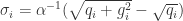
 是随机变量,
 是 scale parameter,
 是 shape parameter。特别地,当
  时,Weibull 分布就是指数分布;当
  时,Weibull 分布就是 Rayleigh 分布。
 ,
, .
. .
. 那么对于每一个
  .
.


 的最大似然估计。第二个式子是关于
  的隐函数,不能够直接求解,需要使用 Newton’s method 来计算。

 ,换言之,
,换言之, 是关于
是关于 

 。如果从一个比较大的数开始的时候,可能使用 Newton 法的时候,会与负轴相交。但是如果从一个较小的数开始,就必定只与正数轴相交。其中 Newton 法的公式是:

 就可以被当作最大似然估计。
 ) yields much better results than a system that uses only unsupervised learning. The context is information security, scanning millions of log entries per day to detect suspicious activity and prevent attacks. Examples of attacks include account takeovers, new account fraud (opening a new account using stolen credit card information), and terms of service abuse (e.g. abusing promotional codes, or manipulating cookies for advantage).


 。从图像上看,一个特征向量可以看成 2 维平面上面的一条线,或者高维空间里面的一个超平面。特征向量所对应的特征值反映了这批数据在这个方向上的拉伸程度。通常情况下,可以把对角矩阵 D 中的特征值进行从大到小的排序,矩阵 P 的每一列也进行相应的调整,保证 P 的第 i 列对应的是 D 的第 i 个对角值。

 是矩阵 P 的前 j 列,也就是说
  是一个 (N,j) 维的矩阵。如果考虑拉回映射的话(也就是从主成分空间映射到原始空间),重构之后的数据集合是
 是使用 top-j 的主成分进行重构之后形成的数据集,是一个 (N,p) 维的矩阵。
 的异常值分数(outlier score)如下:
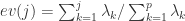
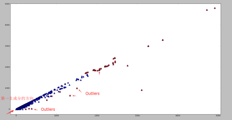
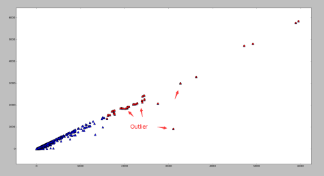
 指的是 Euclidean 范数, ev(j) 表示的是 top-j 的主成分在所有主成分中所占的比例,并且特征值是按照从大到小的顺序排列的。因此,ev(j) 是递增的序列,这就表示 j 越高,越多的方差就会被考虑在 ev(j) 中,因为是从 1 到 j 的求和。在这个定义下,偏差最大的第一个主成分获得最小的权重,偏差最小的最后一个主成分获得了最大的权重 1。根据 PCA 的性质,异常点在最后一个主成分上有着较大的偏差,因此可以获得更高的分数。
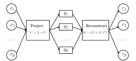
 ,那么可以计算出这 n 个点的均值
  。均值和方差分别被定义为:
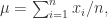

 包含了99.7% 的数据,如果某个值距离分布的均值
  ,那么这个值就可以被简单的标记为一个异常点(outlier)。
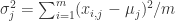
 ,那么可以计算每个维度的均值和方差
  具体来说,对于
  ,可以计算
,可以计算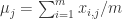
 ,可以计算概率
  如下:
如下:
 ,可以计算 n 维的均值向量
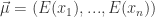
 的协方差矩阵:
![\Sigma=[Cov(x_{i},x_{j})], i,j \in \{1,...,n\}](https://s0.wp.com/latex.php?latex=%5CSigma%3D%5BCov%28x_%7Bi%7D%2Cx_%7Bj%7D%29%5D%2C+i%2Cj+%5Cin+%5C%7B1%2C...%2Cn%5C%7D&bg=ffffff&fg=2b2b2b&s=0&c=20201002)

 是均值向量,那么对于数据集 D 中的其他对象
  ,从
,从 
 是协方差矩阵。
 是数值,可以对这个数值进行排序,如果数值过大,那么就可以认为点
  进行离群点检测,如果
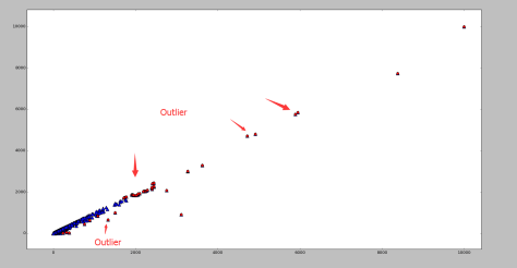
 统计量检测多元离群点
 ,
,
 是
是  是所有对象在第 i 维的均值,n 是维度。如果对象

 ,其中
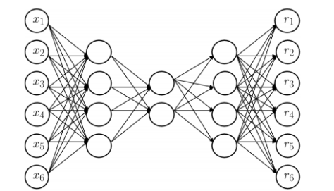
,其中  表示第 k 层中第 i 个神经元的输入,
 表示第 k 层使用的激活函数。那么
 是第 k 层中第 j 个神经元的输出,
 是第 k 层神经元的个数。对于第二层和第四层而言 (k=2,4),激活函数选择为
 是一个参数,通常假设为1。对于中间层 (k=3) 而言,激活函数是一个类阶梯 (step-like) 函数。有两个参数 N 和
  ,N 表示阶梯的个数,
 +
+ .
. ,
, . 那么
. 那么  就如下图所示。
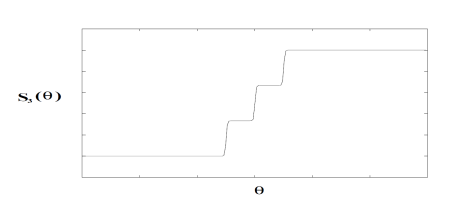
 和
和  。因此有学者指出 [1],使用三个隐藏层是没有必要的,使用1个或者2个隐藏层的神经网络也能够得到类似的结果;同样,没有必要使用
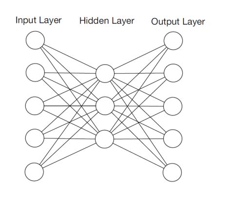
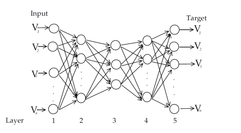
 ,其中有 m 个样本,并且输入和输出是一样的值。换句话说,也就是 n 维向量
 .
.![q=[(n+1)/2]](https://s0.wp.com/latex.php?latex=q%3D%5B%28n%2B1%29%2F2%5D&bg=ffffff&fg=2b2b2b&s=0&c=20201002) ,这里的 [] 表示 Gauss 取整函数。输出层第 j 个神经元的阈值使用
,这里的 [] 表示 Gauss 取整函数。输出层第 j 个神经元的阈值使用  表示,隐藏层第 h 个神经元的阈值使用
  表示。输入层第 i 个神经元与隐藏层第 h 个神经元之间的连接权重是
  , 隐藏层第 h 个神经元与输出层第 j 个神经元之间的连接权重是
  其中
其中 


 是隐藏层第 h 个神经元的输出,
 是激活函数。写成矩阵形式就是:
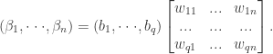
 其中
其中 
 那么直接通过导数计算可以得到
 通过神经网络得到的输出是
  并且
并且  对于
对于  都成立。那么神经网络在训练集
  的均方误差是
 整体的误差是
 +
+
 来获得更新规则,下面来推导每一个参数的更新规则。对于
  计算梯度
计算梯度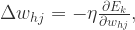
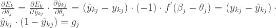
 先影响到第 j 个输出层神经元的输入值
  再影响到第 j 个输出层神经元的输出值
  ,最后影响到
 可以得到
可以得到  对于
对于  可以得到
可以得到 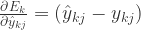 .
. 和
和  可以得到
可以得到 


 .
.


 其中
其中 

 +
+ 并且更新的规则如下:


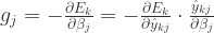
 控制着算法每一轮迭代中的更新步长,若步长太大则容易振荡,太小则收敛速度过慢,需要人工调整学习率。 对每个训练样例,BP 算法执行下面的步骤:先把输入样例提供给输入层神经元,然后逐层将信号往前传,直到计算出输出层的结果;然后根据输出层的误差,再将误差逆向传播至隐藏层的神经元,根据隐藏层的神经元误差来对连接权和阈值进行迭代(梯度下降法)。该迭代过程循环进行,直到达到某个停止条件为止。
 和学习率
和学习率 


 与阈值
与阈值 
 其中 m 是训练集合中样本的个数。不过,标准的 BP 算法每次仅针对一个训练样例更新连接权重和阈值,也就是说,标准 BP 算法的更新规则是基于单个的
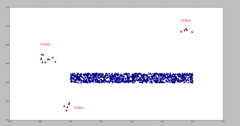
![E=\sum_{i=1}^{K}\sum_{p \in C[i]} dist(p, c[i])^{2}](https://s0.wp.com/latex.php?latex=E%3D%5Csum_%7Bi%3D1%7D%5E%7BK%7D%5Csum_%7Bp+%5Cin+C%5Bi%5D%7D+dist%28p%2C+c%5Bi%5D%29%5E%7B2%7D&bg=ffffff&fg=2b2b2b&s=0&c=20201002)


 上式等价于
上式等价于


 ,意味着学习率是一个正数并且逐渐递减,对每一个维度都是一样的。而在 FTRL 算法里面,每个维度的学习率是不一样的。如果特征 A 比特征 B变化快,那么在维度 A 上面的学习率应该比维度 B 上面的学习率下降得更快。在 FTRL 中,维度 i 的学习率是这样定义的:
 , 所以
, 所以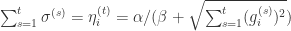
 ,初始化
,初始化  (2)for
 for
for 
 // equals to


 end
end
end
end
 是 sigmoid 函数,
 ,需要预估
,需要预估  ,那么 LogLoss 函数是
 ,
, ,所以 Logistic Regression 的 FTRL 算法就是:
 // gradient of loss function
 , 那么 p(0)=1/3,p(1)=2/3。如果测量的结果是0,那么这个 qubit 的状态就是0,换言之,
 ;如果测量的结果是1,那么这个 qubit 的状态也就变成了1,换言之,
  。
。 ,如果我们对第一个 qubit 使用 Hadamard Gate,那么状态就会变成
 ,其中
,其中 ,
,  。也就是说每一对
  和
和  都会被映射成
  和
和  。因此就证明了,仅仅对 n 个量子比特中的第一位进行了 Hadamard gate 运算,所有的 2^n 个系数都会改变。这个就是在 quantum fourier transform 算法中达到指数级别加速的基础。
 ,
, .
. . Then we have
  ,
,  from the assumption of U. Let
  , we get
 .
.
